Mathematical Formulation
The mathematical development presented here closely parallels that of Zhu and Gelaro (2008). The sensitivity of any functional,  , of the analysis
  or forecast
  can be efficiently computed using the adjoint model which yields information about the gradients of
  and
and  . We can extent the concept of the adjoint sensitivity to compute the sensitivity of the IS4DVAR cost function,
  , in (1) and any other function of the forecast to the observations,
  .
.
In IS4DVAR, we define a quadratic cost function:
 |
(1)
|
where  is the ocean state vector (
 ,
,  ,
,  ,
,  ,
,  ,
, ) with
  ,
,  is the observation error and error of representativeness covariance matrix,
  represents the background error covariance matrix,
  is the innovation vector that represents the difference between the nonlinear background solution (
 ) and the observations,
  . Here,
  is an operator that samples the nonlinear model at the observation location,
  ,
,  is the linearization of , and the operator
  is referred as the tangent linear model propagator.
At the minimum of (1), the cost function gradient  vanishes and:
 |
(2)
|
where  is referred to as the analysis increment, the desired solution of the incremental data assimilation procedure.
The IS4DVAR analysis can be written in the more traditional form as  ( Daley, 1991), where
  , the Kalman gain matrix
  , and
, and  is the Hessian matrix. The entire IS4DVAR procedure is therefore neatly embodied in
  . At the cost function minimum, (1) can be written as
  which yields the sensitivity of the IS4DVAR cost function to the observations.
In the current IS4DVAR/LANCZOS data assimilation algorithm, the cost function minimum of (1) is identified using the Lanczos method (Golub and Van Loan, 1989), in which case:
 |
(3)
|
where  is the matrix of
  orthogonal Lanczos vectors, and
  is a known tridiagonal matrix. Each of the
  iterations of IS4DVAR employed in finding the minimum of yields one column
  of
of  . From (3) we can identify the Kalman gain matrix as
  in which case
  represents the adjoint of the entire IS4DVAR system. The action of
  on the vector
  in (3) can be readily computed since the Lanczos vectors and the matrix are available at the end of each IS4DVAR assimilation cycle.
Therefore, the basic observation sensitivity algorithm is as follows:
- Force the adjoint model with
 to yield
  .
.
- Operate on
 with
with  which is equivalent to a rank
 approximation of the Hessian matrix.
- Integrate the results of step (ii) forward in time using the tangent linear model and save the solution
 . That is, the solution at observation locations.
- Multiply by
 to yield
  .
.
Consider now a forecast  for the interval
 ![t=[t_{0}+\tau ,\;t_{0}+\tau +t_{f}]](https://www.myroms.org/myroms.org/v1/media/math/render/svg/ef32e8e5c9d07811ab0a73354795d9e535b9870b) initialized from
initialized from  obtained from an assimilation cycle over the interval
 ![t=[t_{0},t_{0}+\tau ]](https://www.myroms.org/myroms.org/v1/media/math/render/svg/c96ec79c508db259febecaed385d09338efb6421) , where
, where  is the forecast lead time. In addition, consider
  that depends on the forecast , and which characterizes some future aspect of the forecast circulation. According to the chain rule, the sensitivity
  of to the observations collected during the assimilation cycle is given by:
 |
(4)
|
which again can be readily evaluated using the adjoint model denoted by  and the adjoint of IS4DVAR, .
Technical Description
This ROMS driver can be used to evaluate the impact of each observation on the IS4DVAR data assimilation algorithm by measuring their sensitivity over a specified circulation functional index, . This algorithm is an extension of the adjoint sensitivity driver, AD_SENSITIVITY. As mentioned above, this algorithm is equivalent to taking the adjoint of the IS4DVAR algorithm.
The following steps are carried out in obs_sen_is4dvar.h:
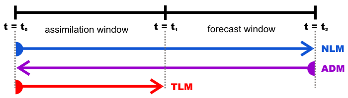
- We begin by running the incremental strong constraint 4DVar data assimilation algorithm (IS4DVAR) with the Lanczos conjugate gradient minimization algorithm (LANCZOS) using inner-loops (
 ) and a single outer-loop (
 ) for the period
 ![t=[t_{0},t_{1}]](https://www.myroms.org/myroms.org/v1/media/math/render/svg/b9bb4f1400e596d7de145eb550cacfb84b388723) . We will denote by
. We will denote by  the background initial condition, and the observations vector by . The resulting Lanczos vectors that we save in the adjoint NetCDF file will be denoted by , where
  .
.
- Next we run the nonlinear model for the combined assimilation plus forecast period
![t=[t_{0},t_{2}]](https://www.myroms.org/myroms.org/v1/media/math/render/svg/adaa0fcd53aefa4c52b806376bba188dd0d23e6f) , where
, where  . This represents the final sweep of the nonlinear model for the period after exiting the inner-loop in the IS4DVAR plus the forecast period
 ![t=[t_{1},t-2]](https://www.myroms.org/myroms.org/v1/media/math/render/svg/84d504d58f842d25f3136fa871447740688312e5) . The initial condition for the nonlinear mode at
. The initial condition for the nonlinear mode at  is and not the new estimated initial conditions,
  . We save the basic state trajectory,
  , of this nonlinear model run for use in the adjoint sensitivity calculation next, and for use in the tangent linear model run later in step (vii). Depending on time for which the sensitivity functional
  is defined, this will dictate
  . For example, if is a functional defined during the forecast interval
  , then
  for this run of the nonlinear model. However, if is defined during the assimilation interval
  , then
  . That is, the definition of should be flexible depending on the choice of .
- The next step involves an adjoint sensitivity calculation for the combined assimilation plus forecast period
![t=[t_{2},t_{0}]](https://www.myroms.org/myroms.org/v1/media/math/render/svg/222f11686198e8170a335f7850fe0770a4c3f723) . The basic state trajectory for this calculation will be that from the nonlinear model run in step (ii).
. The basic state trajectory for this calculation will be that from the nonlinear model run in step (ii).
- After running the regular adjoint sensitivity calculation in (iii), we will have a full 3D-adjoint state vector at time . Let's call this vector . The next thing we want to do is to compute the dot-product of with each of the Lanczos vectors from the previous IS4DVAR run. So if we ran IS4DVAR with inner-loops, we will have Lanczos vectors which we denote as where . So we will compute
 where
where  is the transpose of the vector , and
  for are scalars, so there will be of them.
- The next step is to invert the tridiagonal matrix associated with the Lanczos vectors. Let's denote this matrix as
 . So what we want to solve
  , where
  is the
  vector of scalars from step (iv), and
  is the vector that we want to find. So we solve for
  by using a tridiagonal solver.
- The next step is to compute a weighted sum of the Lanczos vectors. Let's call this
 , where
  for . The
  are obtained from solving the tridiagonal equation in (v), and the are the Lanczos vectors. The vector
  is a full-state vector and be used as an initial condition for the tangent linear model in step (vii).
- Finally, we run the tangent linear model from using from (vi) as the initial conditions. During this run of the tangent linear model, we need to read and process the observations that we used in the IS4DVAR of step 1 and write the solution at the observation points and times to the MODname NetCDF file. The values that we write into this MODname are actually the values multiplied by error covariance assigned to each observation during the IS4DVAR in step (i).
