4DVar Tutorial Introduction: Difference between revisions
No edit summary (change visibility) |
No edit summary (change visibility) |
||
| Line 23: | Line 23: | ||
{|align="center" | {|align="center" | ||
|+style="caption-side:bottom;"|'''Figure 2:''' WC13 Observations | |||
|- | |- | ||
|[[Image:aviso_ssh_2019.png|thumb|400px|<center>'''a)''' Aviso SSH</center>]] | |[[Image:aviso_ssh_2019.png|thumb|400px|<center>'''a)''' Aviso SSH</center>]] | ||
Revision as of 20:49, 24 July 2019
This tutorial shows several examples of ROMS 4D-Var data assimilation algorithms in the California Current System (CCS), 1/3 degree resolution (WC13).
Model Set-up
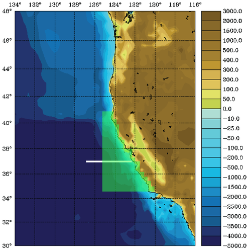
The WC13 model domain is shown in Fig. 1 and has open boundaries along the northern, western, and southern edges of the model domain.

In the tutorial, you will perform a 4D-Var data assimilation cycle that spans the period 3-6 January, 2004. The 4D-Var control vector δz is comprised of increments to the initial conditions, δx(t0), surface forcing, δf(t), and open boundary conditions, δb(t). The prior initial conditions, xb(t0), are taken from the sequence of 4D-Var experiments described by Moore et al. (2010b) in which data were assimilated every 7 days during the period July 2002- December 2004. The prior surface forcing, fb(t), takes the form of surface wind stress, heat flux, and a freshwater flux computed using the ROMS bulk flux formulation, and using near surface air data from COAMPS (Doyle et al., 2009). Clamped open boundary conditions are imposed on (u,v) and tracers, and the prior boundary conditions, bb(t), are taken from the global ECCO product (Wunsch and Heimbach, 2007). The free-surface height and vertically integrated velocity components are subject to the usual Chapman and Flather radiation conditions at the open boundaries. The prior surface forcing and open boundary conditions are provided daily and linearly interpolated in time. Similarly, the increments δf(t) and δb(t) are also computed daily and linearly interpolated in time.
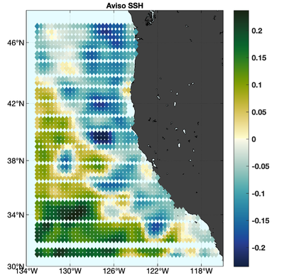
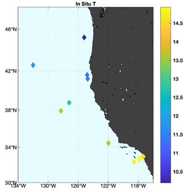
The observations assimilated into the model are satellite SST, satellite SSH in the form of a gridded product from Aviso, and hydrographic observations of temperature and salinity collected from Argo floats and during the GLOBEC/LTOP and CalCOFI cruises off the coast of Oregon and southern California, respectively. The observation locations are illustrated in Fig. 2.
 |
 |
 |
 |
Download Lectures and Exercises
Links to the upcoming 2010 ROMS 4D-Var workshop lectures are provided below. We are planning to record the audio for these lectures to combine with the slides for future reference. These lectures are meant to supplement this 4D-Var tutorial.
- Lecture 1: PDF Primal 4D-Var
- Lecture 2: PDF The Mechanics of 4D-Var
- Lecture 3: PDF Dual 4D-Var
- Lecture 4: PDF 4D-Var Diagnostics
- Lecture 5: PDF Observation Impact and Observation Sensitivity
Below are some of the tutorials pertinent to the upcoming 2010 ROMS 4D-Var workshop:
- Tutorial 1: PDF Explanation of CPP Options, roms.in, s4dvar.in (I4D-Var)
- Tutorial 2: PDF Multiple Outer Loops
- Tutorial 4: PDF Calculation of prior error standard deviations
- Tutorial 5: PDF Explanation of CPP Options, roms.in, s4dvar.in (R4D-Var & 4D-PSAS)
- Tutorial 6: PDF Semi-variograms
- Tutorial 9: PDF Computing normalization coefficients for covariance models
- Tutorial 10: PDF Setting up the impact/sensitivity functional, build script, cpp options and s4dvar.in
- Tutorial 13: PDF Building your observation files
Below are the exercises pertinent to the upcoming 2010 ROMS 4D-Var workshop:
- Exercise 1: PDF Incremental, Strong Constraint 4D-Var
- Exercise 2: PDF I4D-Var with Multiple Outer-loops
- Exercise 3: PDF Dual Formulation 4D-Var: R4D-Var and 4D-PSAS
- Exercise 4: PDF Weak Constraint Dual Formulation 4D-Var
- Exercise 5: PDF Array Modes
- Exercise 6: PDF Observation Impacts
- Exercise 7: PDF Observation Sensitivity
Download Tutorial Files
All of the data files and scripts necessary to run the 4D-Var tests discussed in this tutorial are available from the ROMS Subversion (SVN) repository. To download execute the following command:
Tutorial Directory Structure
When the checkout is complete, you will have the following directory structure under your my_test directory.
 /WC13                               Main California Current System 4D-Var applications
      /ARRAY_MODES                   Stabilized representer matrix array modes and clipping
      /Data                          Input data directory
      /Functionals                   Analytical expressions header files
      /I4DVAR                        Primal form of incremental, strong constraint 4D-Var, I4D-Var
      /Normalization                 4D-Var error covariance normalization coefficients
      /plotting                      4D-Var plotting scripts (Matlab and ROMS plotting package)
      /PSAS                          Dual form of 4D-Var, Physical-space Statistical Analysis System, 4D-PSAS
      /PSAS_analysis_impact          4D-PSAS analysis observation impact
      /PSAS_analysis_sensitivity     4D-PSAS analysis observation sensitivity (adjoint of 4D-PSAS)
Mostly all the directories have a Readme file with detailed instructions for configuring, compiling, running, and plotting the results.
References
The technical description of the algorithms and application used in this tutorial are described in Moore et al. (2010a, b, c).