Vertical S-coordinate: Difference between revisions
Added s-coordinate figure (change visibility) |
m Text replacement - "ocean.in" to "roms.in" (change visibility) |
||
| (45 intermediate revisions by 4 users not shown) | |||
| Line 1: | Line 1: | ||
<div class="title">S-coordinate</div> | <div class="title">Vertical S-coordinate</div> | ||
ROMS has a generalized vertical, terrain-following, coordinate system. Currently, two vertical transformation | |||
equations, <math>z=z(x,y,\sigma,t)</math>, are available which can support numerous vertical stretching 1D-functions when several | |||
constraints are satisfied. | |||
==Transformation Equations== | |||
The following vertical coordinate transformations are available: | |||
<span id="transform1"></span> | |||
{| class="eqno" | |||
|<math display="block">\begin{align}z(x,y,\sigma,t) &= S(x,y,\sigma) + \zeta(x,y,t) \left[1 + \frac{S(x,y,\sigma)}{h(x,y)}\right], \\ | |||
S(x,y,\sigma) &= h_c \, \sigma + \left[h(x,y) - h_c\right] \, C(\sigma) \end{align}</math><!--eqno{(1)}--> | |||
|(1) | |||
|} | |||
or | |||
<span id="transform2"></span> | |||
{| class="eqno" | |||
|<math display="block">\begin{align}z(x,y,\sigma,t) &= \zeta(x,y,t) + \left[\zeta(x,y,t) + h(x,y)\right] \, S(x,y,\sigma), \\ | |||
S(x,y,\sigma) &= \frac{h_c \, \sigma + h(x,y)\, C(\sigma)}{h_c + h(x,y)} \end{align}</math><!--\eqno{(2)}--> | |||
|(2) | |||
|} | |||
where <math> | where <math>S(x,y,\sigma)</math> is a nonlinear vertical transformation functional, <math>\zeta(x,y,t)</math> is the time-varying free-surface, | ||
<math>h(x,y)</math> is the unperturbed water column thickness and <math>z=-h(x,y)</math> corresponds to the ocean bottom, <math>\sigma</math> is a fractional | |||
vertical stretching coordinate ranging from <math>-1 \le\sigma\le 0</math>, <math>C(\sigma)</math> is a nondimensional, monotonic, vertical | |||
stretching function ranging from <math>-1 \le C(\sigma) \le 0</math>, and <math>h_c</math> is a positive thickness controlling the stretching. | |||
In sediment applications, <math>h=h(x,y,t)</math> is changed at every time-step since it is affected by erosion and deposition processes. | |||
:<math> | {{warning}} <span class="red">Warning:</span> We are now very strict about the value of <math>h_{c}</math> and other input vertical transformation parameters. Since the beginning of ROMS, <math>h_c=\min(h_{min},T_{cline})</math> where <math>h_{min}\equiv\hbox{minval}(h)</math> and [[Variables#Tcline | <math>T_{cline}</math>]] is the stretching parameter specified in [[roms.in]]. Notice that it is not possible to build the vertical stretching coordinates when <math>h_{c}> h_{min}</math> and using transformation [[#transform1|(1)]] because it yields <math>\partial{z}/\partial{\sigma} < 0</math> . This has been a legacy issue in ROMS for years, and you are either consistent with the previous set-up of your application or change the value of [[Variables#Tcline | <math>T_{cline}</math>]] in all input NetCDF files and [[roms.in]]. Therefore, in new applications you need to be sure that <math>T_{cline} \le h_{min}</math> when using the transformation [[#transform1|(1)]]. Notice that this restriction is <span class="red">removed</span> in transformation [[#transform1|(2)]] and <math>h_c</math> can be any positive value. It works for both <math>h_c \le h_{min}</math> or <math>h_c > h_{min}</math> . Again, we are now checking internally for all stretching parameters for consistency in all input NetCDF files that have such variables. | ||
We find it convenient to define: | |||
<math display="block"> H_z \equiv {\partial z \over \partial \sigma} </math> | |||
where <math>H_z=H_z(x,y,\sigma,t)</math> are the vertical grid thicknesses. In ROMS, <math>H_z</math> is computed discretely as <math>\Delta z/ \Delta \sigma</math> since this leads to the vertical sum of <math>H_z</math> being exactly the total water column thickness <math>D</math>. | |||
{{note}} Transformation [[#transform1|(1)]] has been available in ROMS since 1999. It is activated by setting [[Variables#Vtransform|Vtransform = 1]] in [[roms.in]]. Notice that, | |||
<math display="block">S(x,y,\sigma) = \begin{cases}0, &\text{if} \;\;\sigma = \;\;\;\,0, \;\; &C(\sigma) = \;\;\;\,0, &\hbox{at the free-surface;}\\ | |||
-h(x,y), &\text{if} \;\;\sigma = -1, \;\; &C(\sigma) = -1, &\hbox{at the ocean bottom.}\end{cases}</math> | |||
In an undisturbed ocean state, corresponding to zero free-surface, <math>z=S(x,y,\sigma)</math>. [[Bibliography#ShchepetkinAF_2005a | Shchepetkin and | |||
McWilliams (2005)]] denotes this transformation as an unperturbed coordinate system since all the depths are not affected by the | |||
displacements of the free-surface. This ensures that the vertical mass fluxes generated by a purely barotropic motion will vanish at every interface | |||
{{note}} Transformation [[#transform2|(2)]] has been available in UCLA-ROMS since 2005. It is activated by setting [[Variables#Vtransform|Vtransform = 2]] in [[roms.in]]. Notice that, | |||
<math display="block">S(x,y,\sigma) = \begin{cases}\;\;0, &\text{if} \;\;\sigma = \;\;\;\,0, \;\; &C(\sigma) = \;\;\;\,0, &\hbox{at the free-surface;}\\ | |||
-1, &\text{if} \;\;\sigma = -1, \;\; &C(\sigma) = -1, &\hbox{at the ocean bottom.}\end{cases}</math> | |||
which is the <math>\sigma | which is different to the behavior of the original functional in [[#transform2|(1)]]. Shchepetkin (personal communication) points out that [[#transform2|(2)]] offers several advantages: | ||
* The | * Regardless of the design of <math>C(\sigma)</math>, it behaves like equally-spaced sigma-coordinates in shallow regions, where <math>h(x,y) \ll h_c</math>. This is advantageous because it avoids excessive resolution and associated CFL limitation is such areas. | ||
* Near-surface refinement behaves more or less like geopotential coordinates in deep regions (level thicknesses, <math>H_z</math>, do not depend or weakly depend on bathymetry), while near-bottom like sigma coordinates (<math>H_z</math> is roughly proportional to depth). This reduces the extreme r-factors near the bottom and reduces pressure gradient errors. | |||
* The '''true''' sigma-coordinate system is recovered as <math>h_c \rightarrow \infty</math>. This is useful when configuring applications with '''flat''' bathymetry and '''uniform''' level thickness. Practically, you can achieve this by setting [[Variables#Tcline|Tcline]] to '''1.0d+16''' in [[roms.in]]. This will set <math>h_c=1.0\hbox{x}10^{16}</math>. Although not necessary, we also recommend that you set <math>\theta_S=0</math> and <math>\theta_B=0</math>.<br> | |||
In an undisturbed ocean state, <math>\zeta\equiv 0</math>, transformation [[#transform2|(2)]] yields the following unperturbed depths, <math>\hat{z}</math>, | |||
{| class="eqno" | |||
|<math display="block"> \hat{z}(x,y,\sigma) \equiv h(x,y) \, S(x,y,\sigma) = h(x,y) \left[\frac{h_c \, \sigma + h(x,y)\, C(\sigma)}{h_c + h(x,y)}\right] </math><!--\eqno{(3)}--> | |||
|(3) | |||
|} | |||
and | |||
{| class="eqno" | |||
|<math display="block"> d\hat{z} = d\sigma \; h(x,y) \; \left[\frac{h_c}{h_c + h(x,y)}\right] </math><!--\eqno{(4)}--> | |||
|(4) | |||
|} | |||
As a consequence, the uppermost grid box retains very little dependency from bathymetry in deep areas, where <math>h_c \ll h(x,y)</math>. | |||
For example, if <math>h_c = 250\,m</math> and <math>h(x,y)</math> changes from <math>2000</math> to <math>6000\,m</math>, the uppermost grid box changes only by a factor | |||
of 1.08 (less than <math>10\%</math>). | |||
==Vertical Stretching Functions== | |||
The above generic vertical transformation design facilitates numerous vertical stretching functions, <math>C(\sigma)</math>. This function | |||
is defined in terms of several parameters which are specified in the standard input file, [[roms.in]]. | |||
'''Stretching Function Properties:''' | |||
* <math>C(\sigma)</math> is a dimensionless, nonlinear, monotonic function; | |||
* <math>C(\sigma)</math> is a continuous differentiable function, or a differentiable piecewise function with smooth transition; | |||
* <math>C(\sigma)</math> must be discretized in terms of the fractional stretched vertical coordinate <math>\sigma</math>, | |||
<math display="block">\sigma(k) = \begin{cases}\frac{k-N}{N}, &\text{at vertical }W\hbox{-points,} &k=0,\dots,N\hbox{,} \\ \\ | |||
\frac{k-N-0.5}{N}, &\text{at vertical }\rho\hbox{-points,} &k=1,\dots,N\end{cases}</math> | |||
* <math>C(\sigma)</math> must be constrained by <math>-1 \le C(\sigma) \le 0</math>, that is, | |||
We | <math display="block">C(\sigma) = \begin{cases}\;\;0, &\text{if} \;\;\sigma = \;\;\;\,0, \;\; &C(\sigma) = \;\;\;\,0, &\hbox{at the free-surface;}\\ | ||
:<math> | -1, &\text{if} \;\;\sigma = -1, \;\; &C(\sigma) = -1, &\hbox{at the ocean bottom.}\end{cases}</math> | ||
'''Available Stretching Functions:''' | |||
<ol> | |||
<li> [[Bibliography#SongY_1994a | Song and Haidvogel (1994)]] function available in ROMS since its beginning, [[Variables#Vstretching|Vstretching = 1]]. <math>C(\sigma)</math> is defined as: | |||
{| class="eqno" | |||
|<math display="block">C(\sigma) = (1 - \theta_B) {\sinh (\theta_S\,\sigma) \over \sinh \theta_S } + | |||
\theta_B \left[{ \tanh [\theta_S ( \sigma + {1\over 2})] \over | |||
2 \tanh ( {1\over 2} \theta_S) } - \frac{1}{2}\right] </math><!--\eqno{(5)}--> | |||
|(5) | |||
|} | |||
where [[Variables#theta_s|<math>{\theta_S}</math>]] and [[Variables#theta_b|<math>\theta_B</math>]] are the surface and bottom control parameters. Their ranges are <math>0 < \theta_S \leq 20</math> and <math>0 \leq \theta_B \leq 1</math>, respectively. This function has the following features: | |||
<ul> | |||
<li>It is infinitely differentiable in <math>\sigma</math>.</li> | |||
<li>The larger the value of <math>{\theta_S}</math>, the more resolution is kept above <math>h_c</math>.</li> | |||
<li>For <math>\theta_B = 0</math>, the resolution all goes to the surface as <math>\theta_S</math> is increased.</li> | |||
<li>For <math>\theta_B = 1</math>, the resolution goes to both the surface and the bottom equally as <math>\theta_S</math> is increased.</li> | |||
<li>For <math>\theta_S \neq 0</math>, there is a subtle mismatch in the discretization of the model equations, for instance in the horizontal viscosity term. We recommend that you stick with ''reasonable'' values of <math>\theta_S</math>, say <math>\theta_S \leq 8</math>.</li> | |||
<li>Some applications turn out to be sensitive to the value of <math>\theta_S</math> used.</li> | |||
</ul> | |||
</li> | |||
<li>A. Shchepetkin (2005) UCLA-ROMS deprecated function, [[Variables#Vstretching|Vstretching = 2]]. <math>C(\sigma)</math> is defined as a piecewise function: | |||
{| class="eqno" | |||
|<math display="block">\begin{align}C(\sigma) &= \mu \, C_{sur}(\sigma) + (1 - \mu) \, C_{bot}(\sigma), \\ \\ C_{sur}(\sigma) &= \frac{1 - \cosh(\theta_S \, \sigma)}{\cosh(\theta_S) - 1}, \qquad \hbox{for }\theta_S > 0, \qquad C_{bot}(\sigma) = \frac{\sinh[\theta_B \,(\sigma + 1)]}{\sinh(\theta_B)} - 1, \qquad \hbox{for }\theta_B > 0, \\ \\ \mu &= (\sigma + 1)^{\alpha} \; \left[1 + \frac{\alpha}{\beta} \left(1 - (\sigma + 1)^{\beta}\right)\right] \end{align}</math><!--\eqno{(6)}--> | |||
|(6) | |||
|} | |||
This function is similar in meaning to the [[Bibliography#SongY_1994a | Song and Haidvogel (1994)]], but note that hyperbolic function in <math>C_{sur}</math> is <math>\cosh</math> instead of <math>\sinh</math> and <br> <math display="block"> \frac {\partial C}{\partial\sigma} \rightarrow 0 \qquad \hbox{as} \;\;\sigma \rightarrow 0.</math></li> | |||
<!--The middle line above should be numbered 6...or maybe the whole group is 6 \eqno{(6)}--> | |||
<!--The middle line below should be numbered 7...or maybe the whole group is 7 \eqno{(7)}--> | |||
<li>R. Geyer function for high bottom boundary layer resolution in relatively shallow applications, [[Variables#Vstretching|Vstretching = 3]]. <math>C(\sigma)</math> is defined as a piecewise function: | |||
{| class="eqno" | |||
|<math display="block">\begin{align}C(\sigma) &= \mu \, C_{bot}(\sigma) + (1 - \mu) \, C_{sur}(\sigma), \\ \\ C_{sur}(\sigma) &= - \frac{\log[\cosh(\gamma\,\hbox{abs}(\sigma)^{\theta_S}] }{\log[\cosh(\gamma)]}, \qquad C_{bot}(\sigma) = \frac{\log[\cosh(\gamma\,(\sigma+1)^{\theta_B}]}{\log[\cosh(\gamma)]} - 1, \\ \\ \mu &= \frac{1}{2} \left[1 - \tanh\left(\gamma\left(\sigma + \frac{1}{2}\right)\right)\right] \end{align}</math> | |||
|(7) | |||
|}where the power exponents [[Variables#theta_s|<math>{\theta_S}</math>]] and [[Variables#theta_b|<math>\theta_B</math>]] are the surface and bottom control parameters specified in standard input file [[roms.in]], as before. Here, <math>\gamma</math> is a scale factor for all hyperbolic functions. Currently, <math>\gamma = 3</math>. Typical values for the control parameters are: | |||
{| border="1" cellspacing="0" cellpadding="5" align="center" | |||
| <math>\theta_S=0.65</math> | |||
| minimal increase of surface resolution | |||
|- | |||
| <math>\theta_S=1.0</math> | |||
| significant surface amplification | |||
|- | |||
| <math>\theta_B=0.58</math> | |||
| no bottom amplification | |||
|- | |||
| <math>\theta_B=1.0</math> | |||
| significant bottom amplification | |||
|- | |||
| <math>\theta_B=1.5</math> | |||
| good bottom resolution for gravity flows | |||
|- | |||
| <math>\theta_B=3.0</math> | |||
| super-high bottom resolution | |||
|- | |||
|}</li><br> | |||
<li>A. Shchepetkin (2010) UCLA-ROMS current function, [[Variables#Vstretching|Vstretching = 4]].<math>C(\sigma)</math> is defined as a continuous, double stretching function: <br><br>Surface refinement function:<span id="equation8"></span> | |||
{| class="eqno" | |||
|<math display="block"> C(\sigma) = \frac{1 - \cosh(\theta_S \, \sigma)}{\cosh(\theta_S) - 1}, \qquad \hbox{for }\theta_S > 0, \qquad C(\sigma) = -{\sigma}^{2}, \qquad \hbox{for }\theta_S \le 0 </math><!--\eqno{(8)}--> | |||
|(8) | |||
|} | |||
Bottom refinement function:<span id="equation9"></span> | |||
{| class="eqno" | |||
|<math display="block"> C(\sigma) = \frac {\exp(\theta_B\,C(\sigma)) - 1} {1 - \exp(-\theta_B)}, \qquad \hbox{for }\theta_B > 0 </math><!--\eqno{(9)}--> | |||
|(9) | |||
|} | |||
Notice that the bottom function [[#equation9|(9)]] is the second stretching of an already stretched transform [[#equation8|(8)]]. The resulting stretching function is continuous with respect to <math>\theta_S</math> and <math>\theta_B</math> as their values approach zero. The range of meaningful values for <math>\theta_S</math> and <math>\theta_B</math> are: <br><br> <math display="block"> 0 \le \theta_S \le 10 \qquad \hbox{and} \qquad 0 \le \theta_B \le 4 </math><br>However, users need to pay attention to extreme r-factor ([[Variables#rx1|rx1]]) values near the bottom. <br><br> {{note}} Due to its functionality and properties [[Variables#Vtransform|Vtransform = 2]] and [[Variables#Vstretching|Vstretching = 4]] are now the default values for ROMS. | |||
</li> | |||
<li>[[Bibliography#SouzaJ_2015 | Souza <i>et al.</i> (2015)]] quadratic Legendre polynomial function, [[Variables#Vstretching|Vstretching = 5]]. The quadratic function allows higher resolution near the surface.<br><br>The fractional stretched vertical coordinate, <math>\sigma</math>, is re-defined as: | |||
<math display="block">\sigma(k) = \begin{cases}-\frac{k^{2} - 2kN + k + N^{2} - N}{N^{2}-N} - \frac{1}{100} \frac{k^{2} - kN}{1 - N}, &\text{at vertical }W\hbox{-points,} &k=0,\dots,N\hbox{,} \\ \\ | |||
-\frac{(k-0.5)^{2} - 2(k-0.5)N + (k-0.5) + N^{2} - N}{N^{2}-N} - \frac{1}{100} \frac{(k-0.5)^{2} - (k-0.5)N}{1 - N}, &\text{at vertical }\rho\hbox{-points,} &k=1,\dots,N\end{cases}</math> | |||
As before, <math>C(\sigma)</math> is defined as a continuous, double stretching function: <br><br>Surface refinement function:<span id="equation8"></span> | |||
{| class="eqno" | |||
|<math display="block"> C(\sigma) = \frac{1 - \cosh(\theta_S \, \sigma)}{\cosh(\theta_S) - 1}, \qquad \hbox{for }\theta_S > 0, \qquad C(\sigma) = -{\sigma}^{2}, \qquad \hbox{for }\theta_S \le 0 </math><!--\eqno{(8)}--> | |||
|(10) | |||
|} | |||
Bottom refinement function:<span id="equation9"></span> | |||
{| class="eqno" | |||
|<math display="block"> C(\sigma) = \frac {\exp(\theta_B\,C(\sigma)) - 1} {1 - \exp(-\theta_B)}, \qquad \hbox{for }\theta_B > 0 </math><!--\eqno{(9)}--> | |||
|(11) | |||
|} | |||
Notice that the bottom function [[#equation11|(11)]] is the second stretching of an already stretched transform [[#equation10|(10)]]. The resulting stretching function is continuous with respect to <math>\theta_S</math> and <math>\theta_B</math> as their values approach zero. The range of meaningful values for <math>\theta_S</math> and <math>\theta_B</math> are: <br><br> <math display="block"> 0 \le \theta_S \le 10 \qquad \hbox{and} \qquad 0 \le \theta_B \le 4 </math><br>However, users need to pay attention to the loss of resolution at the bottom. | |||
</li> | |||
</ol> | |||
==Metadata Considerations== | |||
The above vertical transformations have been registered with the CF Conventions Committee and the NetCDF-Java group. We expect that it will take some time for the CF Committee to approve them. However, the NetCDF-Java is expected to be coded right away. Two new <span class="red">'''standard_name'''</span> variable attributes: <span class="twilightBlue">'''ocean_s_coordinate_g1'''</span> and <span class="twilightBlue">'''ocean_s_coordinate_g2'''</span> have been assigned for transformations [[#transform1|(1)]] and [[#transform2|(2)]], respectively. The terms in the definition are associated with file variables by the <span class="red">'''formula_terms'''</span> attribute as follows: | |||
'''Transformation''' [[#transform1|(1)]]''':''' | |||
<span class="twilightBlue"> double s_rho(s_rho) ; | |||
s_rho:long_name = "S-coordinate at RHO-points" ; | |||
s_rho:valid_min = -1. ; | |||
s_rho:valid_max = 0. ; | |||
s_rho:positive = "up" ; | |||
s_rho:standard_name = "ocean_s_coordinate_g1" ; | |||
s_rho:formula_terms = "s: s_rho C: Cs_r eta: zeta depth: h depth_c: hc" ; | |||
double s_w(s_w) ; | |||
s_w:long_name = "S-coordinate at W-points" ; | |||
s_w:valid_min = -1. ; | |||
s_w:valid_max = 0. ; | |||
s_w:positive = "up" ; | |||
s_w:standard_name = "ocean_s_coordinate_g1" ; | |||
s_w:formula_terms = "s: s_w C: Cs_w eta: zeta depth: h depth_c: hc" ;</span> | |||
'''Transformation''' [[#transform2|(2)]]''':''' | |||
<span class="twilightBlue"> double s_rho(s_rho) ; | |||
s_rho:long_name = "S-coordinate at RHO-points" ; | |||
s_rho:valid_min = -1. ; | |||
s_rho:valid_max = 0. ; | |||
s_rho:positive = "up" ; | |||
s_rho:standard_name = "ocean_s_coordinate_g2" ; | |||
s_rho:formula_terms = "s: s_rho C: Cs_r eta: zeta depth: h depth_c: hc" ; | |||
double s_w(s_w) ; | |||
s_w:long_name = "S-coordinate at W-points" ; | |||
s_w:valid_min = -1. ; | |||
s_w:valid_max = 0. ; | |||
s_w:positive = "up" ; | |||
s_w:standard_name = "ocean_s_coordinate_g2" ; | |||
s_w:formula_terms = "s: s_w C: Cs_w eta: zeta depth: h depth_c: hc" ;</span> | |||
{{note}} Notice that the <span class="red">'''formula_terms'''</span> are identical for both transformations and are independent of the vertical stretching function used. This metadata conventions allows to process/visualize any NetCDF file generated by ROMS easily and correctly compute the associated vertical grid depths. | |||
==Vertical Grid Examples== | |||
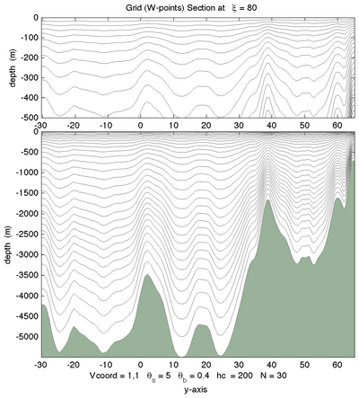
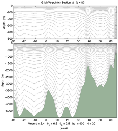
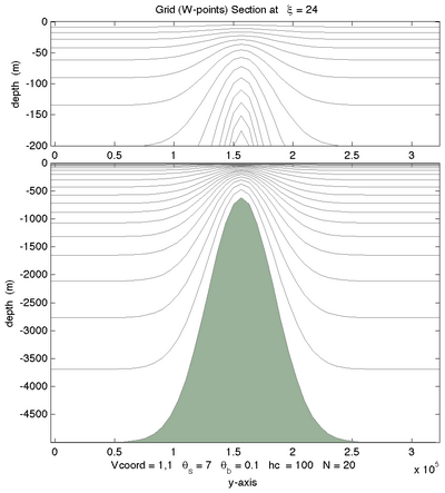
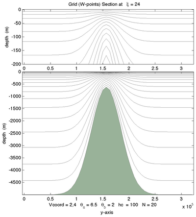
The following figures shows the <math>\sigma</math>-surfaces for both vertical transformations and available vertical stretching functions. These plots were generated in Matlab using the script '''scoord.m'''. | |||
{| | |||
|- | |||
|[[Image:damee4_11.png|thumb|400px|<center>Vtransform=1, Vstretching=1, <math>\theta_S=7.0</math>, <math>\theta_B=0.1</math>, <math>N=30</math></center>]] | |||
|[[Image:damee4_22.png|thumb|400px|<center>Vtransform=2, Vstretching=2, <math>\theta_S=7.0</math>, <math>\theta_B=0.1</math>, <math>N=30</math></center>]] | |||
|} | |||
{| | |||
|- | |||
|[[Image:damee4_24a.png|thumb|400px|<center>Vtransform=2, Vstretching=4, <math>\theta_S=7.0</math>, <math>\theta_B=0.1</math>, <math>N=30</math></center>]] | |||
|[[Image:damee4_24b.png|thumb|400px|<center>Vtransform=2, Vstretching=4, <math>\theta_S=6.5</math>, <math>\theta_B=2.5</math>, <math>N=30</math></center>]] | |||
|} | |||
{| | |||
|- | |||
|[[Image:damee4-15.png|thumb|400px|<center>Vtransform=1, Vstretching=5, <math>\theta_S=6.5</math>, <math>\theta_B=4</math>, <math>N=30</math></center>]] | |||
|[[Image:damee4-25.png|thumb|400px|<center>Vtransform=2, Vstretching=5, <math>\theta_S=6.5</math>, <math>\theta_B=4</math>, <math>N=30</math></center>]] | |||
|} | |||
{| | |||
|- | |||
|[[Image:seamount_11.png|thumb|400px|<center>Vtransform=1, Vstretching=1, <math>\theta_S=7.0</math>, <math>\theta_B=0.1</math>, <math>N=20</math></center>]] | |||
|[[Image:seamount_22.png|thumb|400px|<center>Vtransform=2, Vstretching=2, <math>\theta_S=7.0</math>, <math>\theta_B=0.1</math>, <math>N=20</math></center>]] | |||
|} | |||
{| | |||
|- | |||
|[[Image:seamount_24a.png|thumb|400px|<center>Vtransform=2, Vstretching=4, <math>\theta_S=7.0</math>, <math>\theta_B=0.1</math>, <math>N=20</math></center>]] | |||
|[[Image:seamount_24b.png|thumb|400px|<center>Vtransform=2, Vstretching=4, <math>\theta_S=6.5</math>, <math>\theta_B=2.0</math>, <math>N=20</math></center>]] | |||
|} | |||
{| | |||
|- | |||
|[[Image:seamount_15.png|thumb|400px|<center>Vtransform=1, Vstretching=5, <math>\theta_S=6.5</math>, <math>\theta_B=4</math>, <math>N=20</math></center>]] | |||
|[[Image:seamount_25.png|thumb|400px|<center>Vtransform=2, Vstretching=5, <math>\theta_S=6.5</math>, <math>\theta_B=4</math>, <math>N=20</math></center>]] | |||
|} | |||
:<math> | {| | ||
|- | |||
|[[Image:shelf_11.png|thumb|400px|<center>Vtransform=1, Vstretching=1, <math>\theta_S=1.0</math>, <math>\theta_B=3.0</math>, <math>N=20</math></center>]] | |||
|[[Image:shelf_22.png|thumb|400px|<center>Vtransform=2, Vstretching=2, <math>\theta_S=1.0</math>, <math>\theta_B=3.0</math>, <math>N=20</math></center>]] | |||
|} | |||
{| | |||
|- | |||
|[[Image:shelf_23_b.png|thumb|400px|<center>Vtransform=2, Vstretching=3, <math>\theta_S=1.0</math>, <math>\theta_B=3.0</math>, <math>N=20</math></center>]] | |||
|[[Image:shelf_24.png|thumb|400px|<center>Vtransform=2, Vstretching=4, <math>\theta_S=1.0</math>, <math>\theta_B=4.0</math>, <math>N=20</math></center>]] | |||
|} | |||
Latest revision as of 15:13, 17 July 2019
ROMS has a generalized vertical, terrain-following, coordinate system. Currently, two vertical transformation equations, , are available which can support numerous vertical stretching 1D-functions when several constraints are satisfied.
Transformation Equations
The following vertical coordinate transformations are available:
| (1) |
or
| (2) |
where is a nonlinear vertical transformation functional, is the time-varying free-surface, is the unperturbed water column thickness and corresponds to the ocean bottom, is a fractional vertical stretching coordinate ranging from , is a nondimensional, monotonic, vertical stretching function ranging from , and is a positive thickness controlling the stretching. In sediment applications, is changed at every time-step since it is affected by erosion and deposition processes.
![]() Warning: We are now very strict about the value of and other input vertical transformation parameters. Since the beginning of ROMS, where and is the stretching parameter specified in roms.in. Notice that it is not possible to build the vertical stretching coordinates when and using transformation (1) because it yields . This has been a legacy issue in ROMS for years, and you are either consistent with the previous set-up of your application or change the value of in all input NetCDF files and roms.in. Therefore, in new applications you need to be sure that when using the transformation (1). Notice that this restriction is removed in transformation (2) and can be any positive value. It works for both or . Again, we are now checking internally for all stretching parameters for consistency in all input NetCDF files that have such variables.
Warning: We are now very strict about the value of and other input vertical transformation parameters. Since the beginning of ROMS, where and is the stretching parameter specified in roms.in. Notice that it is not possible to build the vertical stretching coordinates when and using transformation (1) because it yields . This has been a legacy issue in ROMS for years, and you are either consistent with the previous set-up of your application or change the value of in all input NetCDF files and roms.in. Therefore, in new applications you need to be sure that when using the transformation (1). Notice that this restriction is removed in transformation (2) and can be any positive value. It works for both or . Again, we are now checking internally for all stretching parameters for consistency in all input NetCDF files that have such variables.
We find it convenient to define:
where are the vertical grid thicknesses. In ROMS, is computed discretely as since this leads to the vertical sum of being exactly the total water column thickness .
![]() Transformation (1) has been available in ROMS since 1999. It is activated by setting Vtransform = 1 in roms.in. Notice that,
Transformation (1) has been available in ROMS since 1999. It is activated by setting Vtransform = 1 in roms.in. Notice that,
In an undisturbed ocean state, corresponding to zero free-surface, . Shchepetkin and McWilliams (2005) denotes this transformation as an unperturbed coordinate system since all the depths are not affected by the displacements of the free-surface. This ensures that the vertical mass fluxes generated by a purely barotropic motion will vanish at every interface
![]() Transformation (2) has been available in UCLA-ROMS since 2005. It is activated by setting Vtransform = 2 in roms.in. Notice that,
Transformation (2) has been available in UCLA-ROMS since 2005. It is activated by setting Vtransform = 2 in roms.in. Notice that,
which is different to the behavior of the original functional in (1). Shchepetkin (personal communication) points out that (2) offers several advantages:
- Regardless of the design of , it behaves like equally-spaced sigma-coordinates in shallow regions, where . This is advantageous because it avoids excessive resolution and associated CFL limitation is such areas.
- Near-surface refinement behaves more or less like geopotential coordinates in deep regions (level thicknesses, , do not depend or weakly depend on bathymetry), while near-bottom like sigma coordinates ( is roughly proportional to depth). This reduces the extreme r-factors near the bottom and reduces pressure gradient errors.
- The true sigma-coordinate system is recovered as . This is useful when configuring applications with flat bathymetry and uniform level thickness. Practically, you can achieve this by setting Tcline to 1.0d+16 in roms.in. This will set . Although not necessary, we also recommend that you set and .
In an undisturbed ocean state, , transformation (2) yields the following unperturbed depths, ,
| (3) |
and
| (4) |
As a consequence, the uppermost grid box retains very little dependency from bathymetry in deep areas, where . For example, if and changes from to , the uppermost grid box changes only by a factor of 1.08 (less than ).
Vertical Stretching Functions
The above generic vertical transformation design facilitates numerous vertical stretching functions, . This function is defined in terms of several parameters which are specified in the standard input file, roms.in.
Stretching Function Properties:
- is a dimensionless, nonlinear, monotonic function;
- is a continuous differentiable function, or a differentiable piecewise function with smooth transition;
- must be discretized in terms of the fractional stretched vertical coordinate ,
- must be constrained by , that is,
Available Stretching Functions:
- Song and Haidvogel (1994) function available in ROMS since its beginning, Vstretching = 1. is defined as:
(5) where and are the surface and bottom control parameters. Their ranges are and , respectively. This function has the following features:
- It is infinitely differentiable in .
- The larger the value of , the more resolution is kept above .
- For , the resolution all goes to the surface as is increased.
- For , the resolution goes to both the surface and the bottom equally as is increased.
- For , there is a subtle mismatch in the discretization of the model equations, for instance in the horizontal viscosity term. We recommend that you stick with reasonable values of , say .
- Some applications turn out to be sensitive to the value of used.
- A. Shchepetkin (2005) UCLA-ROMS deprecated function, Vstretching = 2. is defined as a piecewise function:
This function is similar in meaning to the Song and Haidvogel (1994), but note that hyperbolic function in is instead of and(6)
- R. Geyer function for high bottom boundary layer resolution in relatively shallow applications, Vstretching = 3. is defined as a piecewise function:
where the power exponents and are the surface and bottom control parameters specified in standard input file roms.in, as before. Here, is a scale factor for all hyperbolic functions. Currently, . Typical values for the control parameters are:(7) minimal increase of surface resolution significant surface amplification no bottom amplification significant bottom amplification good bottom resolution for gravity flows super-high bottom resolution - A. Shchepetkin (2010) UCLA-ROMS current function, Vstretching = 4. is defined as a continuous, double stretching function:
Surface refinement function:(8) Bottom refinement function:
(9) Notice that the bottom function (9) is the second stretching of an already stretched transform (8). The resulting stretching function is continuous with respect to and as their values approach zero. The range of meaningful values for and are:
However, users need to pay attention to extreme r-factor (rx1) values near the bottom.
 Due to its functionality and properties Vtransform = 2 and Vstretching = 4 are now the default values for ROMS.
- Souza et al. (2015) quadratic Legendre polynomial function, Vstretching = 5. The quadratic function allows higher resolution near the surface.
The fractional stretched vertical coordinate, , is re-defined as:As before, is defined as a continuous, double stretching function:
Surface refinement function:(10) Bottom refinement function:
(11) Notice that the bottom function (11) is the second stretching of an already stretched transform (10). The resulting stretching function is continuous with respect to and as their values approach zero. The range of meaningful values for and are:
However, users need to pay attention to the loss of resolution at the bottom.
Metadata Considerations
The above vertical transformations have been registered with the CF Conventions Committee and the NetCDF-Java group. We expect that it will take some time for the CF Committee to approve them. However, the NetCDF-Java is expected to be coded right away. Two new standard_name variable attributes: ocean_s_coordinate_g1 and ocean_s_coordinate_g2 have been assigned for transformations (1) and (2), respectively. The terms in the definition are associated with file variables by the formula_terms attribute as follows:
Transformation (1):
       double s_rho(s_rho) ;
               s_rho:long_name = "S-coordinate at RHO-points" ;
               s_rho:valid_min = -1. ;
               s_rho:valid_max = 0. ;
               s_rho:positive = "up" ;
               s_rho:standard_name = "ocean_s_coordinate_g1" ;
               s_rho:formula_terms = "s: s_rho C: Cs_r eta: zeta depth: h depth_c: hc" ;
       double s_w(s_w) ;
               s_w:long_name = "S-coordinate at W-points" ;
               s_w:valid_min = -1. ;
               s_w:valid_max = 0. ;
               s_w:positive = "up" ;
               s_w:standard_name = "ocean_s_coordinate_g1" ;
               s_w:formula_terms = "s: s_w C: Cs_w eta: zeta depth: h depth_c: hc" ;
Transformation (2):
       double s_rho(s_rho) ;
               s_rho:long_name = "S-coordinate at RHO-points" ;
               s_rho:valid_min = -1. ;
               s_rho:valid_max = 0. ;
               s_rho:positive = "up" ;
               s_rho:standard_name = "ocean_s_coordinate_g2" ;
               s_rho:formula_terms = "s: s_rho C: Cs_r eta: zeta depth: h depth_c: hc" ;
       double s_w(s_w) ;
               s_w:long_name = "S-coordinate at W-points" ;
               s_w:valid_min = -1. ;
               s_w:valid_max = 0. ;
               s_w:positive = "up" ;
               s_w:standard_name = "ocean_s_coordinate_g2" ;
               s_w:formula_terms = "s: s_w C: Cs_w eta: zeta depth: h depth_c: hc" ;
![]() Notice that the formula_terms are identical for both transformations and are independent of the vertical stretching function used. This metadata conventions allows to process/visualize any NetCDF file generated by ROMS easily and correctly compute the associated vertical grid depths.
Notice that the formula_terms are identical for both transformations and are independent of the vertical stretching function used. This metadata conventions allows to process/visualize any NetCDF file generated by ROMS easily and correctly compute the associated vertical grid depths.
Vertical Grid Examples
The following figures shows the -surfaces for both vertical transformations and available vertical stretching functions. These plots were generated in Matlab using the script scoord.m.
 |
 |
 |
 |
 |
 |
 |
 |
 |
 |
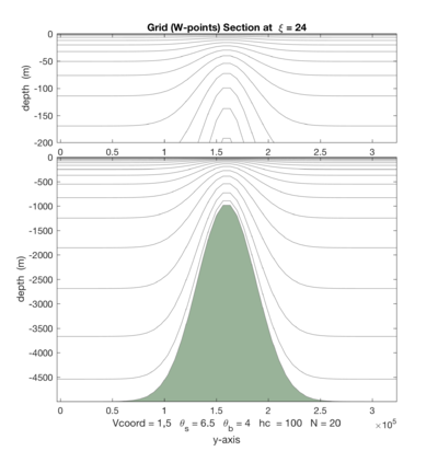 |
 |
 |
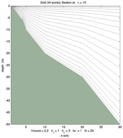 |
 |
 |

![{\displaystyle {\begin{aligned}z(x,y,\sigma ,t)&=S(x,y,\sigma )+\zeta (x,y,t)\left[1+{\frac {S(x,y,\sigma )}{h(x,y)}}\right],\\S(x,y,\sigma )&=h_{c}\,\sigma +\left[h(x,y)-h_{c}\right]\,C(\sigma )\end{aligned}}}](https://www.myroms.org/www.myroms.org/v1/media/math/render/svg/6466f7caf947aba25a5591634397968857c92f81)
![{\displaystyle {\begin{aligned}z(x,y,\sigma ,t)&=\zeta (x,y,t)+\left[\zeta (x,y,t)+h(x,y)\right]\,S(x,y,\sigma ),\\S(x,y,\sigma )&={\frac {h_{c}\,\sigma +h(x,y)\,C(\sigma )}{h_{c}+h(x,y)}}\end{aligned}}}](https://www.myroms.org/www.myroms.org/v1/media/math/render/svg/babbb934465e3692ec8d85fe094a8cd8d664f00f)


![{\displaystyle {\hat {z}}(x,y,\sigma )\equiv h(x,y)\,S(x,y,\sigma )=h(x,y)\left[{\frac {h_{c}\,\sigma +h(x,y)\,C(\sigma )}{h_{c}+h(x,y)}}\right]}](https://www.myroms.org/www.myroms.org/v1/media/math/render/svg/cbfd5c93e7736a3e52b52bd973dbf18e6da9197e)
![{\displaystyle d{\hat {z}}=d\sigma \;h(x,y)\;\left[{\frac {h_{c}}{h_{c}+h(x,y)}}\right]}](https://www.myroms.org/www.myroms.org/v1/media/math/render/svg/73a5c5b5889cee40d3766a46dbe0dcfa0949e8a2)


![{\displaystyle C(\sigma )=(1-\theta _{B}){\sinh(\theta _{S}\,\sigma ) \over \sinh \theta _{S}}+\theta _{B}\left[{\tanh[\theta _{S}(\sigma +{1 \over 2})] \over 2\tanh({1 \over 2}\theta _{S})}-{\frac {1}{2}}\right]}](https://www.myroms.org/www.myroms.org/v1/media/math/render/svg/c14f2fb44197aed4dcf6ec3624e6c467df762995)


![{\displaystyle {\begin{aligned}C(\sigma )&=\mu \,C_{sur}(\sigma )+(1-\mu )\,C_{bot}(\sigma ),\\\\C_{sur}(\sigma )&={\frac {1-\cosh(\theta _{S}\,\sigma )}{\cosh(\theta _{S})-1}},\qquad {\hbox{for }}\theta _{S}>0,\qquad C_{bot}(\sigma )={\frac {\sinh[\theta _{B}\,(\sigma +1)]}{\sinh(\theta _{B})}}-1,\qquad {\hbox{for }}\theta _{B}>0,\\\\\mu &=(\sigma +1)^{\alpha }\;\left[1+{\frac {\alpha }{\beta }}\left(1-(\sigma +1)^{\beta }\right)\right]\end{aligned}}}](https://www.myroms.org/www.myroms.org/v1/media/math/render/svg/f4ed87fed088d3bf7bf480ece2965d96d49f8bbf)


![{\displaystyle {\begin{aligned}C(\sigma )&=\mu \,C_{bot}(\sigma )+(1-\mu )\,C_{sur}(\sigma ),\\\\C_{sur}(\sigma )&=-{\frac {\log[\cosh(\gamma \,{\hbox{abs}}(\sigma )^{\theta _{S}}]}{\log[\cosh(\gamma )]}},\qquad C_{bot}(\sigma )={\frac {\log[\cosh(\gamma \,(\sigma +1)^{\theta _{B}}]}{\log[\cosh(\gamma )]}}-1,\\\\\mu &={\frac {1}{2}}\left[1-\tanh \left(\gamma \left(\sigma +{\frac {1}{2}}\right)\right)\right]\end{aligned}}}](https://www.myroms.org/www.myroms.org/v1/media/math/render/svg/945a7dd7ae17190355eaecac33c1726de1178c01)


