Array Modes Tutorial: Difference between revisions
No edit summary (change visibility) |
No edit summary (change visibility) |
||
| Line 11: | Line 11: | ||
==Introduction== | ==Introduction== | ||
<wikitex>As described in [http://www.myroms.org/tutorials/4DVar_4.pdf Lecture 4], the 4D-Var state-vector increments $\delta{\bf x_a}(t)$ can be expressed as a weighted sum of the array modes: | |||
$$\delta{\bf x_a}(t)=\sum_{i=1}^{M} \lambda_{i}^{-1} ({\bf {\hat{w}}}_{i}^{T} {\bf R}^{-1/2} {\bf d}) {\bf \Psi}_{i} (t)$$ | |||
where ($\lambda_{i},{\bf {\hat{w}}}_i$) are the eigenpairs of the preconditioned stabilized representer matrix (${\bf R}^{-1/2} {\bf GDG}^T {\bf R}^{-1/2} + {\bf I}$). The array modes corresponding to the largest eigenvalue represents the interpolation patterns for the observations that are most stable with respect to changes in the innovation vector '''d''', since the array modes depend ''only'' on the observation locations and not on the observation values.</wikitex> | |||
{{#lst:4DVar_Tutorial_Introduction|setup}} | {{#lst:4DVar_Tutorial_Introduction|setup}} | ||
==Running the Array Modes Driver== | |||
To compute the array modes, you must first run R4D-Var or 4D-PSAS because the array mode driver will use the Lanczos vectors generated by your dual 4D-Var calculation. | |||
To run this exercise, go first to the directory <span class="twilightBlue">WC13/ARRAY_MODES</span>, and follow the directions in the <span class="twilightBlue">Readme</span> file. The only change that you need to make is to '''[[s4dvar.in]]''', where you will select the array mode that you wish to calculate (you may only calculate on mode at a time). The choice of array mode is determined by the parameter [[Variables#Nvct|Nvct]]. The array modes are referenced in reverse order, so choosing [[Variables#Nvct|Nvct]]=[[Variables#Ninner|Ninner]]-1 is the array mode with the second largest eigenvalue, and so on. Note that [[Variables#Nvct|Nvct]] must be assigned a numeric value (''i.e.'' [[Variables#Nvct|Nvct]]=50 for the [[R4D-Var_Tutorial|R4D-Var]] and [[4D-PSAS_Tutorial|4D-PSAS]] tutorials). | |||
{{note}}'''Note:''' Before running the array mode driver, you will need to ensure that you copy the file <span class="twilightBlue">EX3/wc13_mod.nc</span> generated during the [[R4D-Var_Tutorial|R4D-Var]] and [[4D-PSAS_Tutorial|4D-PSAS]] tutorials into <span class="twilightBlue">WC13/R4DVAR</span> or <span class="twilightBlue">WC13/PSAS</span> as appropriate. | |||
==Important CPP Options== | ==Important CPP Options== | ||
The following C-preprocessing options are activated in the [[build_Script|build script]]: | |||
<div class="box"> [[ARRAY_MODES]] Representer Matrix Array Modes driver<br /> [[ARRAY_MODES_SPLIT]] Analysis due to IC, surface forcing, and OBC<br /> [[WC13]] Application CPP option</div> | <div class="box"> [[ARRAY_MODES]] Representer Matrix Array Modes driver<br /> [[ARRAY_MODES_SPLIT]] Analysis due to IC, surface forcing, and OBC<br /> [[WC13]] Application CPP option</div> | ||
==Input NetCDF Files== | ==Input NetCDF Files== | ||
[[WC13]] requires the following input NetCDF files: | |||
<div class="box"> <span class="twilightBlue">Grid File:</span> ../Data/wc13_grd.nc<br /> <span class="twilightBlue">Nonlinear Initial File:</span> wc13_ini.nc<br /> <span class="twilightBlue">Forcing File 01:</span> ../Data/coamps_wc13_lwrad_down.nc<br /> <span class="twilightBlue">Forcing File 02:</span> ../Data/coamps_wc13_Pair.nc<br /> <span class="twilightBlue">Forcing File 03:</span> ../Data/coamps_wc13_Qair.nc<br /> <span class="twilightBlue">Forcing File 04:</span> ../Data/coamps_wc13_rain.nc<br /> <span class="twilightBlue">Forcing File 05:</span> ../Data/coamps_wc13_swrad.nc<br /> <span class="twilightBlue">Forcing File 06:</span> ../Data/coamps_wc13_Tair.nc<br /> <span class="twilightBlue">Forcing File 07:</span> ../Data/coamps_wc13_wind.nc<br /> <span class="twilightBlue">Boundary File:</span> ../Data/wc13_ecco_bry.nc<br /><br /> <span class="twilightBlue">Adjoint Sensitivity File:</span> wc13_ads.nc<br /> <span class="twilightBlue">Initial Conditions STD File:</span> ../Data/wc13_std_i.nc<br /> <span class="twilightBlue">Model STD File:</span> ../Data/wc13_std_m.nc<br /> <span class="twilightBlue">Boundary Conditions STD File:</span> ../Data/wc13_std_b.nc<br /> <span class="twilightBlue">Surface Forcing STD File:</span> ../Data/wc13_std_f.nc<br /> <span class="twilightBlue">Initial Conditions Norm File:</span> ../Data/wc13_nrm_i.nc<br /> <span class="twilightBlue">Model Norm File:</span> ../Data/wc13_nrm_m.nc<br /> <span class="twilightBlue">Boundary Conditions Norm File:</span> ../Data/wc13_nrm_b.nc<br /> <span class="twilightBlue">Surface Forcing Norm File:</span> ../Data/wc13_nrm_f.nc<br/> <span class="twilightBlue">Observations File:</span> wc13_obs.nc<br /> <span class="twilightBlue">Lanczos Vectors File:</span> wc13_lcz.nc</div> | <div class="box"> <span class="twilightBlue">Grid File:</span> ../Data/wc13_grd.nc<br /> <span class="twilightBlue">Nonlinear Initial File:</span> wc13_ini.nc<br /> <span class="twilightBlue">Forcing File 01:</span> ../Data/coamps_wc13_lwrad_down.nc<br /> <span class="twilightBlue">Forcing File 02:</span> ../Data/coamps_wc13_Pair.nc<br /> <span class="twilightBlue">Forcing File 03:</span> ../Data/coamps_wc13_Qair.nc<br /> <span class="twilightBlue">Forcing File 04:</span> ../Data/coamps_wc13_rain.nc<br /> <span class="twilightBlue">Forcing File 05:</span> ../Data/coamps_wc13_swrad.nc<br /> <span class="twilightBlue">Forcing File 06:</span> ../Data/coamps_wc13_Tair.nc<br /> <span class="twilightBlue">Forcing File 07:</span> ../Data/coamps_wc13_wind.nc<br /> <span class="twilightBlue">Boundary File:</span> ../Data/wc13_ecco_bry.nc<br /><br /> <span class="twilightBlue">Adjoint Sensitivity File:</span> wc13_ads.nc<br /> <span class="twilightBlue">Initial Conditions STD File:</span> ../Data/wc13_std_i.nc<br /> <span class="twilightBlue">Model STD File:</span> ../Data/wc13_std_m.nc<br /> <span class="twilightBlue">Boundary Conditions STD File:</span> ../Data/wc13_std_b.nc<br /> <span class="twilightBlue">Surface Forcing STD File:</span> ../Data/wc13_std_f.nc<br /> <span class="twilightBlue">Initial Conditions Norm File:</span> ../Data/wc13_nrm_i.nc<br /> <span class="twilightBlue">Model Norm File:</span> ../Data/wc13_nrm_m.nc<br /> <span class="twilightBlue">Boundary Conditions Norm File:</span> ../Data/wc13_nrm_b.nc<br /> <span class="twilightBlue">Surface Forcing Norm File:</span> ../Data/wc13_nrm_f.nc<br/> <span class="twilightBlue">Observations File:</span> wc13_obs.nc<br /> <span class="twilightBlue">Lanczos Vectors File:</span> wc13_lcz.nc</div> | ||
==Various Scripts and Include Files== | ==Various Scripts and Include Files== | ||
<div class="box"> [[build_Script|build.bash]] bash shell script to compile application<br /> [[build_Script|build.sh]] csh Unix script to compile application<br /> [[job_array_modes|job_array_modes.sh]] job configuration script<br /> <span class="twilightBlue">ocean_wc13.in</span> ROMS standard input script for WC13<br /> [[s4dvar.in]] 4D-Var standard input script template<br /> <span class="twilightBlue">wc13.h</span> WC13 header with CPP options</div> | The following files will be found in <span class="twilightBlue">WC13/ARRAY_MODES</span> directory after downloading from ROMS test cases SVN repository: | ||
<div class="box"> <span class="twilightBlue">Readme</span> Instructions<br /> [[build_Script|build.bash]] bash shell script to compile application<br /> [[build_Script|build.sh]] csh Unix script to compile application<br /> [[job_array_modes|job_array_modes.sh]] job configuration script<br /> <span class="twilightBlue">ocean_wc13.in</span> ROMS standard input script for WC13<br /> [[s4dvar.in]] 4D-Var standard input script template<br /> <span class="twilightBlue">wc13.h</span> WC13 header with CPP options</div> | |||
==Instructions== | ==Instructions== | ||
| Line 30: | Line 45: | ||
#Before you run this application, you need to run the standard [[R4DVAR_Tutorial|R4D-VAR]] ('''../R4DVAR''' directory) since we need the Lanczos vectors. Notice that in [[job_array_modes|job_array_modes.sh]] we have the following operation:<div class="box"><span class="red">cp -p ${Dir}/R4DVAR/wc13_mod.nc wc13_lcz.nc</span></div>In R4D-Var (observartion space minimization), the Lanczos vectors are stored in the output 4D-Var NetCDF file <span class="twilightBlue">wc13_mod.nc</span>. | #Before you run this application, you need to run the standard [[R4DVAR_Tutorial|R4D-VAR]] ('''../R4DVAR''' directory) since we need the Lanczos vectors. Notice that in [[job_array_modes|job_array_modes.sh]] we have the following operation:<div class="box"><span class="red">cp -p ${Dir}/R4DVAR/wc13_mod.nc wc13_lcz.nc</span></div>In R4D-Var (observartion space minimization), the Lanczos vectors are stored in the output 4D-Var NetCDF file <span class="twilightBlue">wc13_mod.nc</span>. | ||
#Customize your preferred [[build_Script|build script]] and provide the appropriate values for: | #Customize your preferred [[build_Script|build script]] and provide the appropriate values for: | ||
#*Root directory, MY_ROOT_DIR | #*Root directory, <span class="salmon">MY_ROOT_DIR</span> | ||
#*ROMS source code, MY_ROMS_SRC | #*ROMS source code, <span class="salmon">MY_ROMS_SRC</span> | ||
#*Fortran compiler, FORT | #*Fortran compiler, <span class="salmon">FORT</span> | ||
#*MPI flags, USE_MPI and USE_MPIF90 | #*MPI flags, <span class="salmon">USE_MPI</span> and <span class="salmon">USE_MPIF90</span> | ||
#*Path of MPI, NetCDF, and ARPACK libraries according to the compiler. Notice that you need to provide the correct places of these libraries for your computer. If you want to ignore this section, comment out the assignment for the variable USE_MY_LIBS. | #*Path of MPI, NetCDF, and ARPACK libraries according to the compiler. Notice that you need to provide the correct places of these libraries for your computer. If you want to ignore this section, comment out the assignment for the variable <span class="salmon">USE_MY_LIBS</span>. | ||
#Notice that the most important CPP options for this application are specified in the [[build_Script|build script]] instead of <span class="twilightBlue">wc13.h</span>:<div class="box"><span class="twilightBlue">setenv MY_CPP_FLAGS "-DARRAY_MODES"<br />setenv MY_CPP_FLAGS "${MY_CPP_FLAGS} -DARRAY_MODES_SPLIT"</span></div>This is to allow flexibility with different CPP options.<div class="para"> </div>For this to work, however, any '''#undef''' directives MUST be avoided in the header file <span class="twilightBlue">wc13.h</span> since it has precedence during C-preprocessing. | #Notice that the most important CPP options for this application are specified in the [[build_Script|build script]] instead of <span class="twilightBlue">wc13.h</span>:<div class="box"><span class="twilightBlue">setenv MY_CPP_FLAGS "-DARRAY_MODES"<br />setenv MY_CPP_FLAGS "${MY_CPP_FLAGS} -DARRAY_MODES_SPLIT"</span></div>This is to allow flexibility with different CPP options.<div class="para"> </div>For this to work, however, any '''#undef''' directives MUST be avoided in the header file <span class="twilightBlue">wc13.h</span> since it has precedence during C-preprocessing. | ||
#You MUST use the [[build_Script|build script]] to compile. | #You MUST use the [[build_Script|build script]] to compile. | ||
| Line 41: | Line 56: | ||
#Execute the configuration [[job_array_modes|job_array_modes.sh]] '''before''' running the model. It copies the required files and creates <span class="twilightBlue">r4dvar.in</span> input script from template '''[[s4dvar.in]]'''. This has to be done '''every time''' that you run this application. We need a clean and fresh copy of the initial conditions and observation files since they are modified by ROMS during execution. | #Execute the configuration [[job_array_modes|job_array_modes.sh]] '''before''' running the model. It copies the required files and creates <span class="twilightBlue">r4dvar.in</span> input script from template '''[[s4dvar.in]]'''. This has to be done '''every time''' that you run this application. We need a clean and fresh copy of the initial conditions and observation files since they are modified by ROMS during execution. | ||
#Run ROMS with data assimilation:<div class="box"><span class="red">mpirun -np 4 oceanM ocean_wc13.in > & log &</span></div> | #Run ROMS with data assimilation:<div class="box"><span class="red">mpirun -np 4 oceanM ocean_wc13.in > & log &</span></div> | ||
==Plotting your Results== | |||
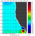
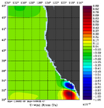
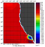
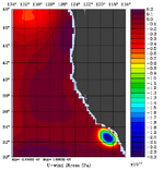
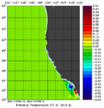
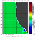
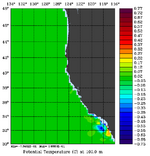
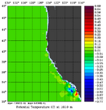
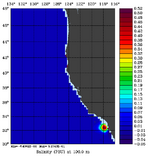
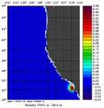
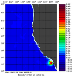
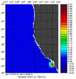
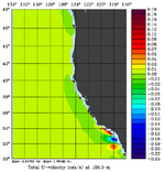
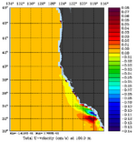
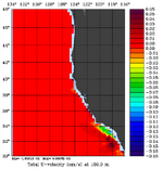
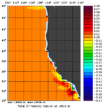
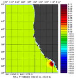
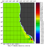
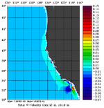
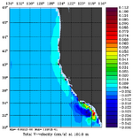
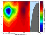
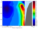
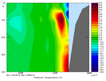
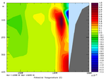
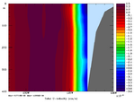
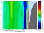
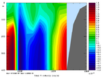
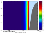
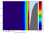
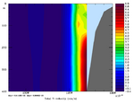
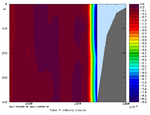
To plot a selection of fields for your chosen array mode, use the Matlab script <span class="twilightBlue">plotting/plot_array_modes.m</span> or ROMS plotting package script <span class="twilightBlue">plotting/ccnt_array_modes.in</span> for horizontal plots at 100 m or <span class="twilightBlue">plotting/csec_arary_modes.in</span> for cross-sections along 37°N. | |||
==Results== | ==Results== | ||
{| | {|align="center" | ||
|- | |- | ||
|[[Image:array_modes_fs_day1.png|thumb|150px|<center>Free-surface Day 1</center>]] | |[[Image:array_modes_fs_day1.png|thumb|150px|<center>Free-surface Day 1</center>]] | ||
| Line 54: | Line 72: | ||
{| | {|align="center" | ||
|- | |- | ||
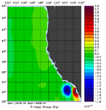
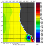
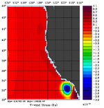
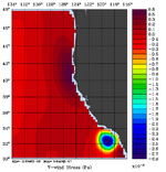
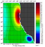
|[[Image:array_modes_uwind_day1.png|thumb|150px|<center>τ<sub>x</sub> Day 1</center>]] | |[[Image:array_modes_uwind_day1.png|thumb|150px|<center>τ<sub>x</sub> Day 1</center>]] | ||
| Line 64: | Line 82: | ||
{| | {|align="center" | ||
|- | |- | ||
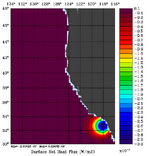
|[[Image:array_modes_vwind_day1.png|thumb|150px|<center>τ<sub>y</sub> Day 1</center>]] | |[[Image:array_modes_vwind_day1.png|thumb|150px|<center>τ<sub>y</sub> Day 1</center>]] | ||
| Line 74: | Line 92: | ||
{| | {|align="center" | ||
|- | |- | ||
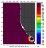
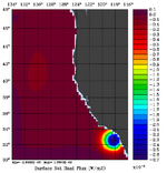
|[[Image:array_modes_heat_day1.png|thumb|150px|<center>Net Heat Flux Day 1</center>]] | |[[Image:array_modes_heat_day1.png|thumb|150px|<center>Net Heat Flux Day 1</center>]] | ||
| Line 84: | Line 102: | ||
{| | {|align="center" | ||
|- | |- | ||
|[[Image:array_modes_T_day1.png|thumb|150px|<center>Temperature Day 1</center>]] | |[[Image:array_modes_T_day1.png|thumb|150px|<center>Temperature Day 1</center>]] | ||
| Line 94: | Line 112: | ||
{| | {|align="center" | ||
|- | |- | ||
|[[Image:array_modes_S_day1.png|thumb|150px|<center>Salinity Day 1</center>]] | |[[Image:array_modes_S_day1.png|thumb|150px|<center>Salinity Day 1</center>]] | ||
| Line 104: | Line 122: | ||
{| | {|align="center" | ||
|- | |- | ||
|[[Image:array_modes_u_day1.png|thumb|150px|<center>U-Momentum Day 1</center>]] | |[[Image:array_modes_u_day1.png|thumb|150px|<center>U-Momentum Day 1</center>]] | ||
| Line 114: | Line 132: | ||
{| | {|align="center" | ||
|- | |- | ||
|[[Image:array_modes_v_day1.png|thumb|150px|<center>V-Momentum Day 1</center>]] | |[[Image:array_modes_v_day1.png|thumb|150px|<center>V-Momentum Day 1</center>]] | ||
| Line 124: | Line 142: | ||
{| | {|align="center" | ||
|- | |- | ||
|[[Image:array_modes_sec_T_day1.png|thumb|150px|<center>Temperature Day 1</center>]] | |[[Image:array_modes_sec_T_day1.png|thumb|150px|<center>Temperature Day 1</center>]] | ||
| Line 134: | Line 152: | ||
{| | {|align="center" | ||
|- | |- | ||
|[[Image:array_modes_sec_S_day1.png|thumb|150px|<center>Salinity Day 1</center>]] | |[[Image:array_modes_sec_S_day1.png|thumb|150px|<center>Salinity Day 1</center>]] | ||
| Line 144: | Line 162: | ||
{| | {|align="center" | ||
|- | |- | ||
|[[Image:array_modes_sec_u_day1.png|thumb|150px|<center>U-Momentum Day 1</center>]] | |[[Image:array_modes_sec_u_day1.png|thumb|150px|<center>U-Momentum Day 1</center>]] | ||
| Line 154: | Line 172: | ||
{| | {|align="center" | ||
|- | |- | ||
|[[Image:array_modes_sec_v_day1.png|thumb|150px|<center>V-Momentum Day 1</center>]] | |[[Image:array_modes_sec_v_day1.png|thumb|150px|<center>V-Momentum Day 1</center>]] | ||
Revision as of 18:15, 2 July 2010
![]() This page is under construction
This page is under construction![]()
Introduction
<wikitex>As described in Lecture 4, the 4D-Var state-vector increments $\delta{\bf x_a}(t)$ can be expressed as a weighted sum of the array modes:
$$\delta{\bf x_a}(t)=\sum_{i=1}^{M} \lambda_{i}^{-1} ({\bf {\hat{w}}}_{i}^{T} {\bf R}^{-1/2} {\bf d}) {\bf \Psi}_{i} (t)$$
where ($\lambda_{i},{\bf {\hat{w}}}_i$) are the eigenpairs of the preconditioned stabilized representer matrix (${\bf R}^{-1/2} {\bf GDG}^T {\bf R}^{-1/2} + {\bf I}$). The array modes corresponding to the largest eigenvalue represents the interpolation patterns for the observations that are most stable with respect to changes in the innovation vector d, since the array modes depend only on the observation locations and not on the observation values.</wikitex>
Model Set-up
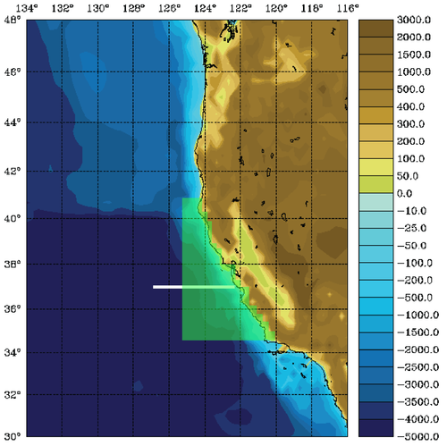
The WC13 model domain is shown in Fig. 1 and has open boundaries along the northern, western, and southern edges of the model domain.
In the tutorial, you will perform a 4D-Var data assimilation cycle that spans the period 3-6 January, 2004. The 4D-Var control vector δz is comprised of increments to the initial conditions, δx(t0), surface forcing, δf(t), and open boundary conditions, δb(t). The prior initial conditions, xb(t0), are taken from the sequence of 4D-Var experiments described by Moore et al. (2011b) in which data were assimilated every 7 days during the period July 2002- December 2004. The prior surface forcing, fb(t), takes the form of surface wind stress, heat flux, and a freshwater flux computed using the ROMS bulk flux formulation, and using near surface air data from COAMPS (Doyle et al., 2009). Clamped open boundary conditions are imposed on (u,v) and tracers, and the prior boundary conditions, bb(t), are taken from the global ECCO product (Wunsch and Heimbach, 2007). The free-surface height and vertically integrated velocity components are subject to the usual Chapman and Flather radiation conditions at the open boundaries. The prior surface forcing and open boundary conditions are provided daily and linearly interpolated in time. Similarly, the increments δf(t) and δb(t) are also computed daily and linearly interpolated in time.
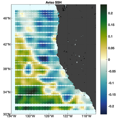
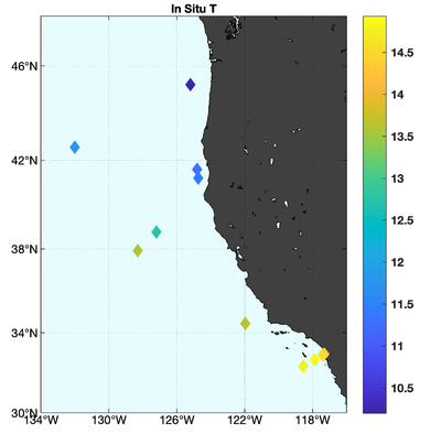
The observations assimilated into the model are satellite SST, satellite SSH in the form of a gridded product from Aviso, and hydrographic observations of temperature and salinity collected from Argo floats and during the GLOBEC/LTOP and CalCOFI cruises off the coast of Oregon and southern California, respectively. The observation locations are illustrated in Fig. 2.
 |
 |
 |
 |
Running the Array Modes Driver
To compute the array modes, you must first run R4D-Var or 4D-PSAS because the array mode driver will use the Lanczos vectors generated by your dual 4D-Var calculation.
To run this exercise, go first to the directory WC13/ARRAY_MODES, and follow the directions in the Readme file. The only change that you need to make is to s4dvar.in, where you will select the array mode that you wish to calculate (you may only calculate on mode at a time). The choice of array mode is determined by the parameter Nvct. The array modes are referenced in reverse order, so choosing Nvct=Ninner-1 is the array mode with the second largest eigenvalue, and so on. Note that Nvct must be assigned a numeric value (i.e. Nvct=50 for the R4D-Var and 4D-PSAS tutorials).
![]() Note: Before running the array mode driver, you will need to ensure that you copy the file EX3/wc13_mod.nc generated during the R4D-Var and 4D-PSAS tutorials into WC13/R4DVAR or WC13/PSAS as appropriate.
Note: Before running the array mode driver, you will need to ensure that you copy the file EX3/wc13_mod.nc generated during the R4D-Var and 4D-PSAS tutorials into WC13/R4DVAR or WC13/PSAS as appropriate.
Important CPP Options
The following C-preprocessing options are activated in the build script:
ARRAY_MODES_SPLIT Analysis due to IC, surface forcing, and OBC
WC13 Application CPP option
Input NetCDF Files
WC13 requires the following input NetCDF files:
Nonlinear Initial File: wc13_ini.nc
Forcing File 01: ../Data/coamps_wc13_lwrad_down.nc
Forcing File 02: ../Data/coamps_wc13_Pair.nc
Forcing File 03: ../Data/coamps_wc13_Qair.nc
Forcing File 04: ../Data/coamps_wc13_rain.nc
Forcing File 05: ../Data/coamps_wc13_swrad.nc
Forcing File 06: ../Data/coamps_wc13_Tair.nc
Forcing File 07: ../Data/coamps_wc13_wind.nc
Boundary File: ../Data/wc13_ecco_bry.nc
Adjoint Sensitivity File: wc13_ads.nc
Initial Conditions STD File: ../Data/wc13_std_i.nc
Model STD File: ../Data/wc13_std_m.nc
Boundary Conditions STD File: ../Data/wc13_std_b.nc
Surface Forcing STD File: ../Data/wc13_std_f.nc
Initial Conditions Norm File: ../Data/wc13_nrm_i.nc
Model Norm File: ../Data/wc13_nrm_m.nc
Boundary Conditions Norm File: ../Data/wc13_nrm_b.nc
Surface Forcing Norm File: ../Data/wc13_nrm_f.nc
Observations File: wc13_obs.nc
Lanczos Vectors File: wc13_lcz.nc
Various Scripts and Include Files
The following files will be found in WC13/ARRAY_MODES directory after downloading from ROMS test cases SVN repository:
build.bash bash shell script to compile application
build.sh csh Unix script to compile application
job_array_modes.sh job configuration script
ocean_wc13.in ROMS standard input script for WC13
s4dvar.in 4D-Var standard input script template
wc13.h WC13 header with CPP options
Instructions
To run this application you need to take the following steps:
- We need to run the model application for a period that is long enough to compute meaningful circulation statistics, like mean and standard deviations for all prognostic state variables (zeta, u, v, T, and S). The standard deviations are written to NetCDF files and are read by the 4D-Var algorithm to convert modeled error correlations to error covariances. The error covariance matrix, D, is very large and not well known. It is modeled as the solution of a diffusion equation as in Weaver and Courtier (2001).In this application, we need standard deviations for initial conditions, surface forcing (ADJUST_WSTRESS and ADJUST_STFLUX), and open boundary conditions (ADJUST_BOUNDARY). The standard deviations for the initial and open boundary conditions are in terms of the unbalanced error covariance (K Du KT) since the balanced operator is activated (BALANCE_OPERATOR and ZETA_ELLIPTIC).The balance operator imposes a multivariate constraint on the error covariance such that the unobserved variable information is extracted from observed data by establishing balance relationships (i.e., T-S empirical formulas, hydrostactic balance, and geostrophic balance) with other state variables (Weaver et al., 2005).These standard deviations have already been created for you:../Data/wc13_std_i.nc initial conditions
../Data/wc13_std_b.nc open boundary conditions
../Data/wc13_std_f.nc surface forcing (wind stress and net heat flux) - Since we are modeling the error covariance matrix, D, we need to compute the normalization coefficients to ensure that the diagonal elements of the associated correlation matrix C are equal to unity. There are two methods to compute normalization coefficients: exact and randomization (an approximation).The exact method is very expensive on large grids. The normalization coefficients are computed by perturbing each model grid cell with a delta function scaled by the area (2D state variables) or volume (3D state variables), and then by convolving with the squared-root adjoint and tangent linear diffusion operators.The approximate method is cheaper: the normalization coefficients are computed using the randomization approach of Fisher and Courtier (1995). The coefficients are initialized with random numbers having a uniform distribution (drawn from a normal distribution with zero mean and unit variance). Then, they are scaled by the inverse squared-root of the cell area (2D state variable) or volume (3D state variable) and convolved with the squared-root adjoint and tangent diffusion operators over a specified number of iterations, Nrandom.Check following parameters in the 4D-Var input script s4dvar.in (see input script for details):Nmethod == 0 ! normalization methodThese normalization coefficients have already been computed for you (../Normalization) using the exact method since this application has a small grid (54x53x30):
Nrandom == 5000 ! randomization iterations
LdefNRM == F F F F ! Create a new normalization files
LwrtNRM == F F F F ! Compute and write normalization
CnormI(isFsur) = T ! 2D variable at RHO-points
CnormI(isUbar) = T ! 2D variable at U-points
CnormI(isVbar) = T ! 2D variable at V-points
CnormI(isUvel) = T ! 3D variable at U-points
CnormI(isVvel) = T ! 3D variable at V-points
CnormI(isTvar) = T T ! NT tracers
CnormB(isFsur) = T ! 2D variable at RHO-points
CnormB(isUbar) = T ! 2D variable at U-points
CnormB(isVbar) = T ! 2D variable at V-points
CnormB(isUvel) = T ! 3D variable at U-points
CnormB(isVvel) = T ! 3D variable at V-points
CnormB(isTvar) = T T ! NT tracers
CnormF(isUstr) = T ! surface U-momentum stress
CnormF(isVstr) = T ! surface V-momentum stress
CnormF(isTsur) = T T ! NT surface tracers flux../Data/wc13_nrm_i.nc initial conditionsNotice that the switches LdefNRM and LwrtNRM are all false (F) since we already computed these coefficients.
../Data/wc13_nrm_b.nc open boundary conditions
../Data/wc13_nrm_f.nc surface forcing (wind stress and
net heat flux)The normalization coefficients need to be computed only once for a particular application provided that the grid, land/sea masking (if any), and decorrelation scales (HdecayI, VdecayI, HdecayB, VdecayV, and HdecayF) remain the same. Notice that large spatial changes in the normalization coefficient structure are observed near the open boundaries and land/sea masking regions. - Before you run this application, you need to run the standard R4D-VAR (../R4DVAR directory) since we need the Lanczos vectors. Notice that in job_array_modes.sh we have the following operation:cp -p ${Dir}/R4DVAR/wc13_mod.nc wc13_lcz.ncIn R4D-Var (observartion space minimization), the Lanczos vectors are stored in the output 4D-Var NetCDF file wc13_mod.nc.
- Customize your preferred build script and provide the appropriate values for:
- Root directory, MY_ROOT_DIR
- ROMS source code, MY_ROMS_SRC
- Fortran compiler, FORT
- MPI flags, USE_MPI and USE_MPIF90
- Path of MPI, NetCDF, and ARPACK libraries according to the compiler. Notice that you need to provide the correct places of these libraries for your computer. If you want to ignore this section, comment out the assignment for the variable USE_MY_LIBS.
- Notice that the most important CPP options for this application are specified in the build script instead of wc13.h:setenv MY_CPP_FLAGS "-DARRAY_MODES"This is to allow flexibility with different CPP options.
setenv MY_CPP_FLAGS "${MY_CPP_FLAGS} -DARRAY_MODES_SPLIT"For this to work, however, any #undef directives MUST be avoided in the header file wc13.h since it has precedence during C-preprocessing. - You MUST use the build script to compile.
- Customize the ROMS input script ocean_wc13.in and specify the appropriate values for the distributed-memory partition. It is set by default to:Notice that the adjoint-based algorithms can only be run in parallel using MPI. This is because of the way that the adjoint model is constructed.
- Customize the configuration script job_array_modes.sh and provide the appropriate place for the substitute Perl script:set SUBSTITUTE=${ROMS_ROOT}/ROMS/Bin/substituteThis script is distributed with ROMS and it is found in the ROMS/Bin sub-directory. Alternatively, you can define ROMS_ROOT environmental variable in your .cshrc login script. For example, I have:setenv ROMS_ROOT /home/arango/ocean/toms/repository/trunk
- Execute the configuration job_array_modes.sh before running the model. It copies the required files and creates r4dvar.in input script from template s4dvar.in. This has to be done every time that you run this application. We need a clean and fresh copy of the initial conditions and observation files since they are modified by ROMS during execution.
- Run ROMS with data assimilation:mpirun -np 4 oceanM ocean_wc13.in > & log &
Plotting your Results
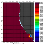
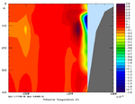
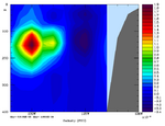
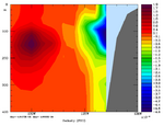
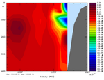
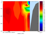
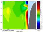
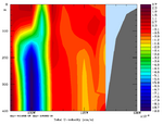
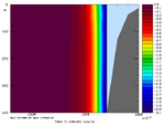
To plot a selection of fields for your chosen array mode, use the Matlab script plotting/plot_array_modes.m or ROMS plotting package script plotting/ccnt_array_modes.in for horizontal plots at 100 m or plotting/csec_arary_modes.in for cross-sections along 37°N.
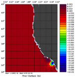
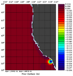
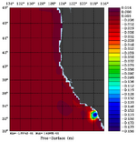
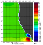
Results
 |
 |
 |
 |
 |
 |
 |
 |
 |
 |
 |
 |
 |
 |
 |
 |
 |
 |
 |
 |
 |
 |
 |
 |
 |
 |
 |
 |
 |
 |
 |
 |
 |
 |
 |
 |
 |
 |
 |
 |
 |
 |
 |
 |
 |
 |
 |
 |
 |
 |
 |
 |
 |
 |
 |
 |
 |
 |
 |
 |
References
The technical description of the algorithms and application used in this tutorial are described in Moore et al. (2010a, b, c).