easygrid: Difference between revisions
No edit summary (change visibility) |
No edit summary (change visibility) |
||
| Line 14: | Line 14: | ||
==Download EASYGRID== | ==Download EASYGRID== | ||
*[http://easygrid4roms.googlecode.com/files/EASYGRID_v1.rar '''Download EASYGRID'''] | *[http://easygrid4roms.googlecode.com/files/EASYGRID_v1.rar '''Download EASYGRID''']<small> (This download also includes, bathymetry, coastline and other files required for this tutorial)</small> | ||
*Extract (i.e. unzip or unpack) the file in a location where it can stay indefinitely. | *Extract (i.e. unzip or unpack) the file in a location where it can stay indefinitely. | ||
*Add the location where you placed EASYGRID to your Matlab search path <small>(see [[MEXNC#How to install MEXNC?|#5]] as an example).</small> | *Add the location where you placed EASYGRID to your Matlab search path <small>(see [[MEXNC#How to install MEXNC?|#5]] as an example).</small> | ||
| Line 263: | Line 263: | ||
==Editing Masks== | ==Editing Masks== | ||
After you created your grid.nc file, you will likely need to edit the mask. That is, you will need to change some land-pixes of the mask into sea-pixels... and vice versa. | After you created your grid.nc file, you will likely need to edit the mask. That is, you will need to change some land-pixes of the mask into sea-pixels... and vice versa. To edit your grid's mask, you can use <span class="red">editmask.m</span> , which is a GUI script included in the [[MEXNC#How to install ROMS Matlab tool-kit?|ROMS Matlab tool-kit]] (inside the rmask directory). | ||
{| style="width:100%; background:LightYellow; margin-top:10px; border:1px solid red;" cellpadding="1" cellspacing="0" | {| style="width:100%; background:LightYellow; margin-top:10px; border:1px solid red;" cellpadding="1" cellspacing="0" | ||
| Line 282: | Line 272: | ||
<br> | <br> | ||
Here are step-by-step instructions: | '''Here are step-by-step instructions to use <span class="red">editmask.m</span>:''' | ||
* Start | *Start the GUI by typing in Matlab's Command Window: | ||
editmask | editmask | ||
* Select the NetCDF grid file to edit (<span class="red">Fjord_grd.nc</span> in this tutorial) | * Select the NetCDF grid file to edit (<span class="red">Fjord_grd.nc</span> in this tutorial) | ||
* Select the .mat coastline file associated to the grid file (<span class="red">Fjord_coast.mat</span> in this tutorial) | * Select the .mat coastline file associated to the grid file (<span class="red">Fjord_coast.mat</span> in this tutorial) | ||
[[image:Fjord_editmask1.jpg|right|800px|]] | |||
[[image:Fjord_editmask1.jpg| | * Select "Set Land" ("Edit Mode" section on the right) and <span class="red">mask 1-cell bays</span> like the examples circled in A and B. | ||
* Proceed to <span class="red">mask disconnected lakes</span>, like one in example circled in E. | |||
* Although tiny islands apparently don't cause troubles... you may want to select "Set Sea" and unmask "islands" that you consider unrealistic or unnecessary, like the ones circled by C and D. | |||
* Once you finished editing the mask, <span class="red">CLICK SAVE</span>. This will update your NetCDF grid file for ROMS. | |||
* Close GUI. | |||
===Masking Criteria=== | |||
* Fill in (i.e. mask) 1-cell bays | |||
* Fill in disconnected lakes | |||
* Tiny islands apparently don't cause troubles. | |||
<br> | <br> | ||
<br> | <br> | ||
<br> | <br> | ||
Revision as of 23:13, 21 April 2008
April 21, 2008 |
EASYGRID is a simple matlab script to make ROMS grids and initialization files. It is a austere grid-making alternative designed as a beginner's tool. Since most of EASYGRID is in one file (easygrid.m), it is easier to understand the steps required to generate a simple grid (i.e. useful as a learning or teaching tool) and also reduces the required steps to get the software up and running (i.e. downloading and compiling dependencies)... hence you can play with grid-making and ROMS-running earlier in the game.
This WikiROMS page is a tutorial, where I provide test bathymetry and coastline so you can play with EASYGRID. Also, this page is where I will post notes and updates.
Download EASYGRID
- Download EASYGRID (This download also includes, bathymetry, coastline and other files required for this tutorial)
- Extract (i.e. unzip or unpack) the file in a location where it can stay indefinitely.
- Add the location where you placed EASYGRID to your Matlab search path (see #5 as an example).
- Dependencies: EASYGRID uses MEXNC, SNCTOOLS and ROMS Matlab tool-kit (only a few scripts like spheric_dist.m , smth_bath.m , pcolorjw.m).
 For a tutorial on how to download/install dependencies, CLICK HERE.
Get bathymetry
EASYGRID needs a bathymetry .mat file containing 3 vectors (xbathy, ybathy and zbathy), where:
- xbathy = longitude
- ybathy = latitude
- zbathy = depth (positive, in meters... For more information about bathymetry for ROMS, click HERE)
 NOTE: Vectors xbathy and ybathy are in decimal degrees.
There easiest way to get bathymetry data (that I know) is to use Rich Signell's read_srtm30plus.m Matlab script. Instant bathymetry in 1 line of Matlab code! Click HERE for instructions to get and use read_srtm30plus.m.

The most difficult way to get bathymetry data (that I know) is to scan a chart and then digitize it using your mouse and a digitizing software like Didger (sorry, I am not aware of any good digitizing free software).
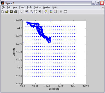
For this tutorial, you will need Fjord_bathy.mat . You should already have this file since it is included in the EASYGRID_v1.rar file that you downloaded above. I created Fjord_bathy.mat by merging two bathymetry files... one high-resolution digitized from a chart and another coarser-resolution using read_srtm30plus.m (see Figure).
![]() If you want to reproduce this plot as an exercise, copy-paste the following code on Matlab's Command Window:
If you want to reproduce this plot as an exercise, copy-paste the following code on Matlab's Command Window:
load Fjord_bathy.mat
plot(xbathy,ybathy,'.');
xlabel('Longitude');
ylabel('Latitude');
axis square;
Getting coastline
In EASYGRID, the coastline is only used for plotting and it therefore not indispensable. However, a later step of mask editing (using editmask.m) requires a coastline file. For both, EASYGRID and editmask.m, the coastline should be 2 vectors named "lat" and "lon" (both in units of decimal degrees) contained in a .mat file.

An easy way to get coastline data is at NOAA's Coastline Extractor. Remember to select Matlab as format option (not default). SEAGRID's WikiROMS page has excellent information on how to use the Coastline Extractor, and tools to correct and manipulate coastline data.
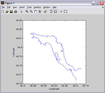
For this tutorial, you will need Fjord_coast.mat . You should already have this file since it is included in the EASYGRID_v1.rar file that you downloaded above. I created Fjord_coast.mat from the digitized chart I use to make the bathymetry file (see Figure).
![]() If you want to reproduce this plot as an exercise, copy-paste the following code on Matlab's Command Window:
If you want to reproduce this plot as an exercise, copy-paste the following code on Matlab's Command Window:
load Fjord_coast.mat
plot(lon,lat);
xlabel('Longitude');
ylabel('Latitude');
axis square;
Making your grid
Set up USER SETTINGS
Before you run EASYGRID to create your ROMS grid, you need to edit EASYGRID's user settings, which is the first part of script (after the help lines). Beside each entry line there are detailed instructions. In fact, most of the "user-manual" for EASYGRID is included within itself. Therefore I will simply copy-paste below a snippet from EASYGRID's code that contains the USER SETTINGS/instructions section.
![]() NOTE: The default settings in EASYGRID are for the Fjord test case, hence you can just run EASYGRID (using the included Fjord_bathy.mat and Fjord_coast.mat files) to generate the grid and initial-conditions files required for the Fjord test case tutorial.
NOTE: The default settings in EASYGRID are for the Fjord test case, hence you can just run EASYGRID (using the included Fjord_bathy.mat and Fjord_coast.mat files) to generate the grid and initial-conditions files required for the Fjord test case tutorial.
%*******************************************************************************************************************************
% USER SETTINGS ****************************************************************************************************************
%*******************************************************************************************************************************
%
% Switches -------------------------
     save_grid = 1;   % Save GRID in a NetCDF file ( yes = 1; no = 0 )
     save_init = 1;   % Create (and save) INITIAL CONDITIONS (from grid) ( yes = 1; no = 0 )
 screen_output = 1;   % Displays (on the screen) many parameters that need to be copy-pasted in the ocean.in file ( yes = 1; no = 0 )
     plot_grid = 1;   % Plot grid ( yes = 1; no = 0 )
   smooth_grid = 1;   % Smooth bathymetry ( yes = 1; no = 0 ) using H. Arango's smth_bath.m , which applies a Shapiro filter to the bathymetry
%
% -------------------------------------------------------------------------
% GRID SETTINGS -----------------------------------------------------------
% -------------------------------------------------------------------------
%
% Geographical and Grid parameters --------
     lat =  44.8125;        % Latitude  (degrees) of the bottom-left corner of the grid.
     lon = -62.8855;        % Longitude (degrees) of the bottom-left corner of the grid.
%
       X = 9100;            % Width of domain (meters)
       Y = 2550;            % Length of domain (meters)
rotangle = -43;             % Angle (degrees) to rotate the grid conterclock-wise
   resol = 30;              % Cell width and height (i.e. Resolution)in meters. Grid cells are forced to be (almost) square.
       N = 10;              % Number of vertical levels
%
%
% Bathymetry -------------- % Bathymetry for ROMS is measured positive downwards (zeros are not allowed) see: https://www.myroms.org/wiki/index.php/Grid_Generation#Bathymetry
                            % To allow variations in surface elevation (eg. tides) while keeping all depths positive,
                            % an arbitrary offset (see minh below) is added to the depth vector.
%
      hh = nan;             % Analytical Depth (meters) used to create a uniform-depth grid. If using a bathymetry file, leave hh = nan;
    minh = 4;               % Arbitrary depth offset in meters (see above). minh should be a little more than the maximum expected tidal variation.
   Bathy = 'Test_bathy.mat';% Bathymetry file. If using the analytical depth above (i.e. hh ~= nan), then Bathy will not be used.
                            % The bathymetry file should be a .mat file containing 3 vectors (xbathy, ybathy and zbathy). where xbathy = Longitude,
                            % ybathy = Latitude and zbathy = depth (positive, in meters). xbathy and ybathy are in decimal degrees See: http://en.wikipedia.org/wiki/Decimal_degrees
       %Bathymetry smoothing routine...  See "Switches section" (above) to turn this ON or OFF
       if smooth_grid == 1;
           order = 2;       % Order of Shapiro filter (2,4,8)... default: 2
            rlim = 0.35;    % Maximum r-factor allowed (0.35)... default: 0.35
           npass = 50;      % Maximum number of passes.......... default: 50
       end
%---------------------------------
%
%
% Coastline ----------------------
   Coast = load('Test_coast.mat'); % If there isn't a coastline file... comment-out this line: e.g. %Coast = load('test_coast.mat');
                                   % The coastline is only used for plotting. The coastline .mat file should contain 2 vectors named "lat" and "lon"
%
%
% -------------------------------------------------------------------------
% OUTPUT: File naming and NetCDF descriptors ------------------------------
% -------------------------------------------------------------------------
Grid_filename = 'Fjord';      % Filename for grid and initial conditions files (don't include extension).
                              % "_grd.nc" is added to grid file and "_ini.nc" is added to initial conditions file
Descrip_grd   = 'Test grid';               %Description for grid .nc file
Descrip_ini   = 'Test initial conditions'; %Description for initial conditions .nc file
Author        = 'John Smith';
Computer      = 'My Computer';
%
% -------------------------------------------------------------------------
% INITIAL CONDITIONS ------------------------------------------------------
% -------------------------------------------------------------------------
if save_init == 1; % See "Switches section" (above) to turn this ON or OFF
    % Initial conditions will be constant throught the grid domain
    %--------------------------------------------------------------------------
    NH4          = 0.1;     % Ammonium concentration (millimole_NH4 meter-3)
    NO3          = 10;      % Nitrate concentration (millimole_N03 meter-3)
    chlorophyll1 = 0.3;     % Chlorophyll concentration in small phytoplankyon (milligrams_chlorophyll meter-3)
    chlorophyll2 = 0.3;     % Chlorophyll concentration in large phytoplankyon (milligrams_chlorophyll meter-3)
    detritus1    = 0.03;    % Small detritus concentration (millimole_nitrogen meter-3)
    detritus2    = 0.03;    % Large detritus concentration (millimole_nitrogen meter-3)
    detritusC1   = 1;       % Small detritus carbon concentration (millimole_carbon meter-3)
    detritusC2   = 0.2;     % Large detritus carbon concentration (millimole_carbon meter-3)
    phyto1       = 0.02;    % Small phytoplankton concentration (millimole_nitrogen meter-3)
    phyto2       = 0.02;    % Large phytoplankton concentration (millimole_nitrogen meter-3)
    phytoC1      = 0.2;     % Small phytoplankton carbon concentration (millimole_carbon meter-3)
    phytoC2      = 0.1;     % Small phytoplankton carbon concentration (millimole_carbon meter-3)
    salt         = 30;      % Salinity (PSU)
    temp         = 9;       % Potential temperature (Celsius)
    u            = 0;       % u-momentum component (meter second-1)
    ubar         = 0;       % Vertically integrated u-momentum component (meter second-1)
    v            = 0;       % v-momentum component (meter second-1)
    vbar         = 0;       % Vertically integrated v-momentum component (meter second-1)
    zeta         = 0;       % Free-surface (meters)
    zooplankton  = 0.01;    % Zooplankton concentration "millimole_nitrogen meter-3"
    zooplanktonC = 0.5;     % Zooplankton carbon concentration "millimole_carbon meter-3"
    %--------------------------------------------------------------------------
end
%
%
%
%*******************************************************************************************************************************
% END OF USER SETTINGS *********************************************************************************************************
%*******************************************************************************************************************************
Geographical/Grid parameters
After you got the bathymetry and coastline of your study region, now it is time to place a grid on it... In the USER SETTINGS section, you have to specify lat lon X Y and rotangle. This is done in an iterative manner, where first you input your best-guesses, then you plot the grid. From the plot you can adjust your geographical/grid parameters... plot... adjust... plot... adjust... and so on.
![]() You may want to turn off some switches (see below) to speed up the plotting process.
You may want to turn off some switches (see below) to speed up the plotting process.
% Switches -------------------------
     save_grid = 0;   % Save GRID in a NetCDF file ( yes = 1; no = 0 )
     save_init = 0;   % Create (and save) INITIAL CONDITIONS (from grid) ( yes = 1; no = 0 )
 screen_output = 0;   % Displays (on the screen) many parameters that need to be copy-pasted in the ocean.in file ( yes = 1; no = 0 )
     plot_grid = 1;   % Plot grid ( yes = 1; no = 0 )
   smooth_grid = 0;   % Smooth bathymetry ( yes = 1; no = 0 ) using H. Arango's smth_bath.m , which applies a Shapiro filter to the bathymetry
Bathymetry smoothing
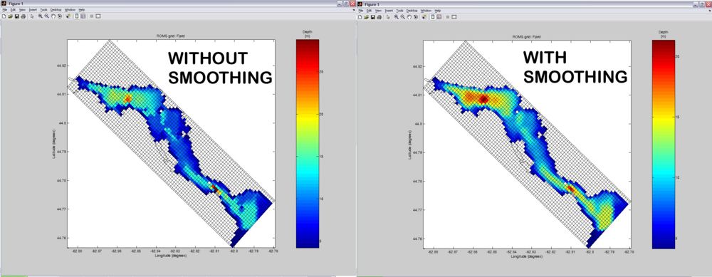
ROMS doesn't like rough bathymetry with abrupt changes in topography. Therefore, after you got your grid where you wanted it to be, the next step is to smooth the bathymetry. Turn ON the smooth_grid variable in the %Switches section. Usually simply enabling smoothing (with the default settings) will do a pretty good job. But if unsatisfied, you can iteratively tweak the parameters in the %Bathymetry somoothing section of the USER SETTINGS until obtaining the desired smoothness. Below is a comparison of grids without and with smoothing (default settings).

Initial Conditions
ROMS initial-conditions NetCDF files contain information on the spatial distribution of one (or multiple) variable(s) that ROMS uses at the START of the simulation. The value of each initialization variable is specified for each corresponding cell in the ROMS grid... hence, inside a typical initial-conditions file, there will be one three-dimensional matrix (matching grid dimensions) for each specified variable. EASYGRID can generate Initial-Conditions NetCDF files for ROMS, however, only in a rudimentary manner... the user can only choose a single value for each initial-condition variable... EASYGRID makes each initial-conditions variable constant over the entire grid domain. This may be only useful in some simple cases and to do "quick-tests".
To change the value of a initial-condition variable, simply go to the INITIAL CONDITIONS section in the USER SETTINGS and change the value of the variable of interest.
If you need to add another initial-condition variable... (1) add in the INITIAL CONDITIONS section of the USER SETTINGS:
new_variable = 0; % Variable description (units)
and (2) add the following snippet to the end of the easygrid.m file (substitute the parts in red)
%--------------------------------------------------------------------------
       dims                    = { 'time'; 's_rho'; 'eta_rho'; 'xi_rho'};
       nc{ 'newvar'}           = ncdouble(dims);
       nc{ 'newvar'}(:,:,:)    = ones(N,Mp,Lp).* 'new_variable';
       nc{ 'newvar'}.time      = 'ocean_time' ;
Parameter output on screen
If screen_output is turned ON (in the USER SETTINGS sections), EASYGRID will output some parameters to screen. Make sure you write this numbers (Lm, MM, N and DT) since you will need to enter them in the ocean.in file prior to running ROMS.
|  COPY-PASTE the following parameters into your ocean.in file
|  ----------------------------------------------------------------------------------------------
|
|
|     Lm == 90         ! Number of I-direction INTERIOR RHO-points
|     Mm == 24         ! Number of J-direction INTERIOR RHO-points
|      N == 10         ! Number of vertical levels
|
|
|  Make sure the Baroclinic time-step (DT) in your ocean.in file is less than: 3.3882 seconds
|  ----------------------------------------------------------------------------------------------
- The parameters Lm, Mm and N are the basically the dimensions of the RHO grid.
- The parameter DT is the baroclinic time-step and it should be less than SQRT( (dx^2+dy^2)/(g*h(x,y) ). You can read a bit more about this in the this forum post (middle of page).
Saving .nc files
Once you got your grid in place, your bathymetry smoothed and your initial-conditions adjusted... it is time to save the NetCDF files for ROMS. To do this, simply turn on ALL the Switches in the USER SETTING section and run EASYGRID. Besides the plot, this time it will also save the grid and initial conditions .nc files. EASYGRID will also output some parameters to screen. ![]() Make sure you write down this numbers (Lm, MM, N and DT), since you will need to enter them in the ocean.in file prior to running ROMS.
Make sure you write down this numbers (Lm, MM, N and DT), since you will need to enter them in the ocean.in file prior to running ROMS.
Editing Masks
After you created your grid.nc file, you will likely need to edit the mask. That is, you will need to change some land-pixes of the mask into sea-pixels... and vice versa. To edit your grid's mask, you can use editmask.m , which is a GUI script included in the ROMS Matlab tool-kit (inside the rmask directory).
Here are step-by-step instructions to use editmask.m:
- Start the GUI by typing in Matlab's Command Window:
editmask
- Select the NetCDF grid file to edit (Fjord_grd.nc in this tutorial)
- Select the .mat coastline file associated to the grid file (Fjord_coast.mat in this tutorial)

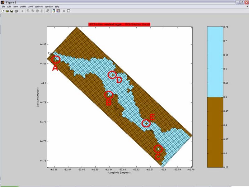
- Select "Set Land" ("Edit Mode" section on the right) and mask 1-cell bays like the examples circled in A and B.
- Proceed to mask disconnected lakes, like one in example circled in E.
- Although tiny islands apparently don't cause troubles... you may want to select "Set Sea" and unmask "islands" that you consider unrealistic or unnecessary, like the ones circled by C and D.
- Once you finished editing the mask, CLICK SAVE. This will update your NetCDF grid file for ROMS.
- Close GUI.
Masking Criteria
- Fill in (i.e. mask) 1-cell bays
- Fill in disconnected lakes
- Tiny islands apparently don't cause troubles.

