Custom Query (986 matches)

I implemented the changes made by Ufuk Turunçoğlu to cmeps_roms.F, now called cmeps_roms.h, to avoid interference with the native framework. The native ROMS NUOPC cap module is now called esmf_roms.h. Either NUOPC module is included in esmf_roms.F via CPP. The coupling interface for CDEPS/CMEPS is activated with the CMEPS option, and is intended for connecting to the ​UFS-coastal framework.

For now, the UFS-coastal repository is downloaded from:

git -c submodule.ADCIRC.update=none clone -b feature/coastal_app --recursive https://github.com/oceanmodeling/ufs-coastal

Notice that we are omitting the ADCIRC component during the cloning since it is still private and working with the research branch feature/coastal_app. This coupling capability is still under development and is complex. Thus, it is not ready for the regular user. We are currently testing the interface to connect ROMS to the UFS coupling framework.

An ESM/build_ufs.sh is provided to facilitate configuring and compiling any ROMS application. It is currently configured for the Hurricane Irene (IRENE) application. See ​roms_test for more information. It works for the ROMS-DATA coupling system using the CDEFS connectors or the CMEPS mediator. The DATA component is replacing the atmosphere model, and it tests ROMS connection to CDEPS, CMEPS, and UFS coupling driver.

LAPACK/ARPACK Legacy Library:

The ARPACK and its MPI-based parallel (PARPACK) version are well-tested libraries to solve large eigenvalue matrix problems. Our primary use in ROMS is to use its Implicit Restarted Arnoldi Method (IRAM) to solve for the Ritz eigenfunctions in several of our Tangent and Adjoint-based propagators that are part of the Generalized Linear Stability (GLS) package described in Moore et al. (2004) Ocean Modelling paper ​https://doi.org/10.1016/j.ocemod.2003.11.001. As far as I know, we cannot use a modern replacement library. Therefore, we will continue using that library when running any of the drivers of the GLS package.

However, the ARPACK library includes selected Linear Algebra functions from the BLAS and LAPACK libraries. In particular, we use LAPACK's DSTEQR function to solve for the eigenvalues/eigenvectors of the tri-diagonal system used in the various 4D-Var minimizations available in ROMS.

Thus, I spent some time looking for a replacement. It turns out that any modern software out there is built on top of LAPACK (Phyton, MATLAB, R, SciPy, and others). There are also bindings to C and C++. We could use the eigen, written in C++, but it will be complicated since I will have to write and test the inter-operability mechanism in ROMS for C++ to Fortran 2003 and vice versa (Fortran 2003 to C++). It turns out that the libeigen has BLAS and LAPACK components. See: ​https://gitlab.com/libeigen/eigen. On top of that, there are reports that the eigen library is much slower than Fortran libraries. Thus, I am giving up on the eigen library. It is beyond our scope.

I decided to adapt the functions we need from LAPACK into module lapack_mod.F, which I converted to Fortran 2003. It includes a total of 19 LAPACK functions. I modernized the code, which had initially 41 GOTOs. I managed to remove 18 of them. The remaining 23 are located in the function DSTEQR. I was able to get identical 4D-Var solutions during testing. That eigenfunction solver is tricky, and removing the remaining GOTOs is dangerous.

The complicated GOTOs are still in selected functions but can be removed from the final C-preprocessing file (lapack_mod.f90) by activating the CPP option REMOVE_LAPACK_GOTOS. For example, in the function DLASRT used to sort the eigenvalues, I have:

#ifdef REMOVE_LAPACK_GOTOS
            DecLOOP_3 : DO                           ! forever LOOP 3
              DecLOOP_1 : DO                         ! forever LOOP 1
                J = J - 1
                IF (D(J) .GE. DMNMX) EXIT DecLOOP_1  ! terminate LOOP 1
              END DO DecLOOP_1
!
              DecLOOP_2 : DO                         ! forever LOOP 2
                I = I + 1
                IF (D(I) .LE. DMNMX) EXIT DecLOOP_2  ! terminate LOOP 2
              END DO DecLOOP_2
!
              IF (I .LT. J) THEN
                TMP = D(I)
                D(I) = D(J)
                D(J) = TMP
                CYCLE DecLOOP_3                      ! iterate LOOP 3
              ELSE
                EXIT DecLOOP_3                       ! terminate LOOP 3
              END IF
            END DO DecLOOP_3
#else
   60       CONTINUE
   70       CONTINUE
            J = J - 1
            IF (D(J) .LT. DMNMX) GO TO 70
   80       CONTINUE
            I = I + 1
            IF (D(I) .GT. DMNMX) GO TO 80
            IF (I .LT. J) THEN
              TMP = D(I)
              D(I) = D(J)
              D(J) = TMP
              GO TO 60
            END IF
#endif

Notice that the above piece of code is slightly complicated. It requires knowledge of the modern Fortran Standard and Objective-Oriented Programming principles to remove the GOTOs, which were unavailable in Fortran and compilers over 40 years ago. This doesn't imply that the LAPACK library is incorrect and produces the wrong results. I am keeping the original code with the GOTOs for reference and testing.

We no longer need the LAPACK/ARPACK libraries to run any 4D-Var drivers in ROMS because the functions that we need are available in our modern adaptation module lapack_mod.F.

Many thanks to Ufuk Turunçoğlu for his hard work and help connecting ROMS to the UFS-coastal.

GitHub Pull Request: ​https://github.com/myroms/roms/pull/25

In 4D-Var, the background (prior) error covariance, B, is a large matrix that cannot be computed or stored directly. Still, its effects can be modeled using spatial correlations, C, and spatial convolutions via diffusion operators. To convert correlations into error covariance, we multiply by a diagonal matrix of the background error standard deviations, S. Hence,

B = L S C S^T L^T

where L is a balance operator, if BALANCE_OPERATOR is activated in ROMS. It allows the information on unobserved state variables to be extracted from directly observed quantities by imposing linear balance relationships between temperature and other state variables using T-S empirical formulas, the linear equation of state, hydrostatic balance, and geostrophic balance. Please check Moore et al. (2011) for more information.

This update includes an approach to computing the standard deviation, S, directly from the background state field as an alternative to climatological values read from the input NetCDF files. It follows the work of Mogensen et al. (2012) by assuming the background errors are proportional to the vertical derivatives of the background field. The field error has a similar profile shape, but the difference with the actual error values is due to a vertical displacement.

In the past, the standard deviation was read from input NetCDF files and computed from a long simulation of the ROMS application. The climatological S can be categorized as monthly, seasonal, or annual values.

The modeling of the standard deviation from the background (prior) is activated with the STD_MODEL option and done in the new module background_std.F. For further information about this capability in ROMS, check Moore et al. (2020).

New parameters are added to 4D-Var input script s4dvar.in to constraint the standard deviation profile at the mixed-layer depth and deep ocean:

! Modeled standard deviation (STD) of Background Error Covariance parameters.
!
! The Mogensen et al. (2012) formulation assumes that the background errors
! are proportional to vertical derivatives of the state vector field. Its
! error has a similar field profile shape, but the difference with its
! ture error value is due to a vertical displacement.
!
! If COMPUTE_MLD is activated, the mixed-layer depth is computed using the
! criterion from Kara et al. (2000). Otherwise, it will be set to a uniform
! value provided below.

Sigma_max(isFsur) == 0.025d0           ! free surface  maximum STD value

Sigma_max(isUvel) == 0.06d0            ! U-velocity maximum STD value
 Sigma_ml(isUvel) == 0.05d0            ! U-velocity minimum STD at mixed layer
 Sigma_do(isUvel) == 0.02d0            ! U-velocity minimum STD in deep ocean
 Sigma_dz(isUvel) == 500.0d0           ! U-velocity vertical displacement

Sigma_max(isVvel) == 0.06d0            ! V-velocity maximum STD
 Sigma_ml(isVvel) == 0.05d0            ! V-velocity minimum STD at mixed layer
 Sigma_do(isVvel) == 0.02d0            ! V-velocity minimum STD in deep ocean
 Sigma_dz(isVvel) == 500.0d0           ! V-velocity vertical displacement

Sigma_max(isTvar) == 0.33d0   0.056d0  ! 1:NT tracers maximum STD
 Sigma_ml(isTvar) == 0.05d0   0.05d0   ! 1:NT tracers minimum STD at the mixed layer
 Sigma_do(isTvar) == 0.02d0   0.0028d0 ! 1:NT tracers minimum STD in the deep ocean
 Sigma_dz(isTvar) == 40.0d0   40.0d0   ! 1:NT tracer vertical displacement

      mld_uniform == -75.0d0           ! Uniform mixed layer depth value

Notice we have the option COMPUTE_MLD to compute the mixed-layer depth using the approach of Kara et al. (2000) or set a constant value of mld_uniform.

Two new routines are added, def_std.F and wrt_std.F, to write the standard deviation modeled from the background into an output NetCDF file. It will be needed in the split 4D-Var algorithms and for postprocessing. The new filename is also specified in s4dvar.in:

! If computing the standard deviation from the background (prior) state
! vector as an alternative to climatological values read from the
! input NetCDF file, enter the output standard deviation file name,
! [1:Ngrids].

       STDnameC == roms_std_c.nc

We foresee enhancing this capability in the future. We only model the standard deviation for adjusting the initial state vector (zeta, u, v, T, and S). We don't have options for background error on the model (weak constraint), lateral model boundary conditions, surface tracer fluxes, and surface momentum stress. Thus, those standard deviation values are still read from input files.

Notice that the standard deviation structure for I/O management increased its inner dimension from 4 to 5 in mod_iounits.F:

       IF (.not.allocated(STD)) THEN
         allocate ( STD(5,Ngrids) )
       END IF

WARNING:

• The s4dvar.in has the additional parameters mentioned above. Please update your 4D-Var input script to use his new capability.

References:

• Kara A., P. Rochford, and E. Hulburt, 2000: An optimal definition for ocean mixed layer depth, J. Geophys. Res., 105, NoC7, pp 16, 803-16, 821.

• Mogensen, K., M.A. Balmaseda, and A.T. Weaver, 2012: The NEMOVAR ocean data assimilation system implemented in the ECMWF ocean analysis for system 4, ECMWF Tech. Memorandum 668, 59.

• Moore, A.M., H.G. Arango, G. Broquet, B.S. Powell, A.T. Weaver, and J. Zavala-Garay, 2011: The Regional Ocean Modeling System (ROMS) 4-dimensional variational data assimilations systems, Part I - System overview and formulation, Prog. Oceanogr., 91, 34-49, ​https://doi:10.1016/j.pocean.2011.05.004.

• Moore, A., J. Zavala-Garay, H.G. Arango, C.A. Edwards, J. Anderson, and T. Hoar, 2020: Regional and basin scale applications of ensemble adjustment Kalman filter and 4D-Var ocean data assimilation systems, Progress in Oceanography, 189, 102450, ​https://doi.org/10.1016/j.pocean.2020.102450.

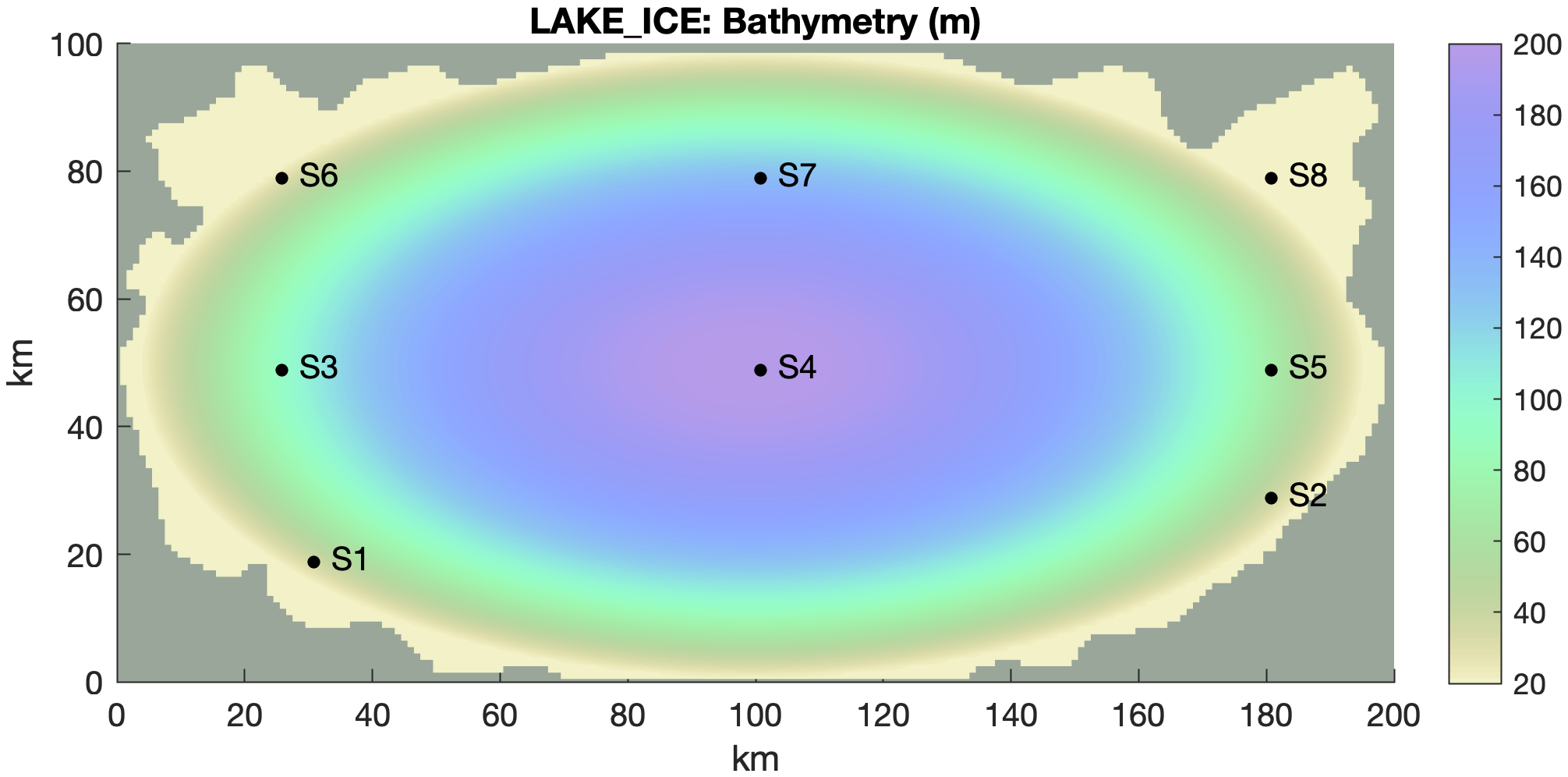
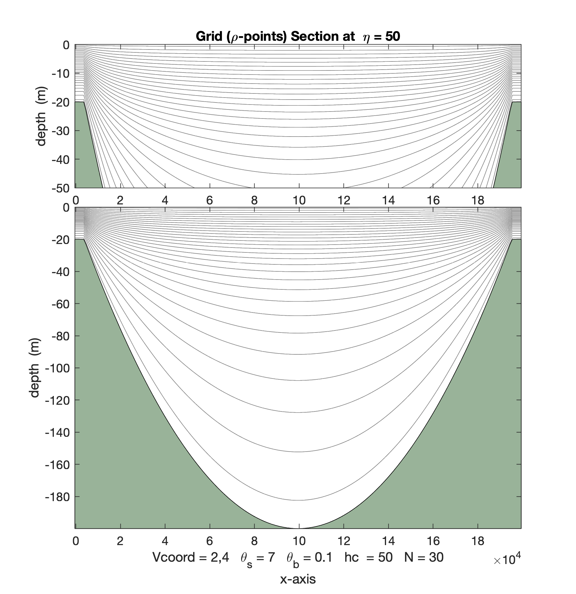
The ROMS Native Sea Model was updated and tested with the LAKE_ICE test case. It is an idealized application 200x100x30 at 1km resolution:

The location of the output stations is denoted as S1, S2, S3, S4, S5, S6, S7, and S8 and used to store the time series of the solution at hourly intervals. The vertical grid is well resolved in the upper 20m with a bathymetry range between 20-200m.

ROMS is initialized on Jan-1-2010 and runs for 800 days until Apr-13-2012. Please check the following link for more information, instructions, and solution plots:

​https://github.com/myroms/roms_test/blob/main/lake_ice/Forward/Readme.md

• Many thanks to Scott Durski for updating and improving the existing sea ice model, which was initially written by Paul Budgell and maintained and documented by Kate Hedstrom.

• Many thanks to Mike Dinniman for his help in debugging and testing this new version of the sea ice model.