Custom Query (986 matches)
Results (499 - 501 of 986)
| Ticket | Owner | Reporter | Resolution | Summary |
|---|---|---|---|---|
| #609 | Done | Spatially varying Jerlov water type | ||
| Description |
Added the option to have spatially varying Jerlov water types for light absorption in the water column. This is used when SOLAR_SOURCE or LMD_SKPP CPP options are activated. A new CPP option WTYPE_GRID is introduced to activate spatially varying Jerlov water types. The ROMS internal variable Jwtype is now a floating-point variable to facilitate I/O manipulation within the metadata model. The spatially varying Jerlov water type index can be specified in two ways:
The variable Jwtype is used in lmd_swfrac to compute the fraction of shortwave flux penetrating the water column (light absorption), modeled as a double exponential decay function in Jerlov water type. The double exponential parameters (lmd_mu1, lmd_mu2, lmd_r1) were also enhanced to add additional Jerlov coastal water types: 1, 3, 5, 7. Currently, the following Jerlow water types are supported: Array Jerlov
Index Water Type Examples
----- ---------- --------
1 I Open Pacific
2 IA Eastern Mediterranean, Indian Ocean
3 IB Western Mediterranean, Open Atlantic
4 II Coastal waters, Azores
5 III Coastal waters, North Sea
6 1 Skagerrak Strait
7 3 Baltic
8 5 Black Sea
9 7 Coastal waters, dark
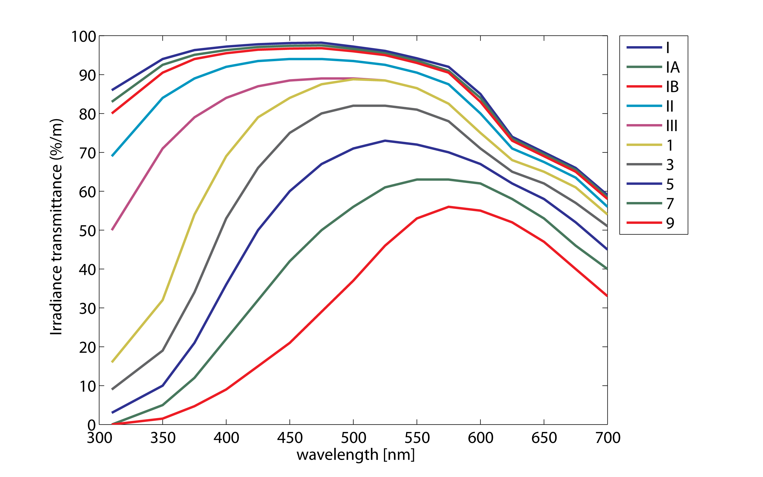
The range of indices 1:9 are ordered by increasing absorption: from clear water (type I) to dark turbidity water (type 7). The indices correspond to the paramenters (lmd_mu1, lmd_mu2, lmd_r1) used to model the light absorption into the water column using a double exponential fitting function of (Paulson and Simpson, 1997). The following figure shows the Jerlov's water type classification based on transmittance along 1 m of seawater: The water type 9 was not included in the above array classification indices because its double exponential fitting parameters are not available. I also introduced routine ana_dqdsst.h to specify the surface net heat flux sentivity to SST, d(Q)/d(SST), with analytical expressions (internal ROMS variable dqdt). This is activated with new CPP option ANA_DQDSST. It is now possible to specify the SST in a NetCDF forcing file and the d(Q)/d(SST) field with an analytical function. No longer we need both variables in the NetCDF file. I haven't coded the function that computes d(Q)/d(SST) using the formula reported in Barnier et al. (1995). Several additional atmospheric field are required (see their equation 6b). The values for d(Q)/d(SST) can be negative or positive and has units of Watts meters-2 Celsius-1 (or internal kinematic units of m/s/Celsius). If you are planning to use QCORRECTION in your application, I suggest you to read Barnier et al. (1995) paper first. There are some messages in the forum suggesting the summer warming trends cannot be fixed with QCORRECTION. I just tried in the Gulf of Mexico and it worked well. It is just a matter how you specify the appropriate d(Q)/d(SST) values. I usually use monthly composite SST from the NOAA CoastWatch OpenDAP catalog (http://oceanwatch.pfeg.noaa.gov/thredds/catalog.html), see product SST, Blended, Global, EXPERIMENTAL (BA/ssta/mday). Reference: Barnier, B., L. Siefridt, and P. Marchesiello, 1995: Thermal forcing for a global ocean circulation model using a three-year climatology of ECMWF analyses, J. Marine Systems, 6, 363-380. |
|||
| #610 | Done | IMPORTANT: Updated input multi-file capabities | ||
| Description |
Multi-files are allowed in ROMS for several input fields. That is, the time records for a particular input field can be split into several NetCDF files. For example, we can have in ocean.in: BRYNAME == ../../Data/g/gom_nwa_bry_2006_g.nc |
../../Data/g/gom_nwa_bry_2007_g.nc |
../../Data/g/gom_nwa_bry_2008_g.nc |
../../Data/g/gom_nwa_bry_2009_g.nc |
../../Data/g/gom_nwa_bry_2010_g.nc |
../../Data/g/gom_nwa_bry_2011_g.nc |
../../Data/g/gom_nwa_bry_2012_g.nc
NFFILES == 9 ! number of unique forcing files
FRCNAME == ../../Data/Forcing/gom_sms_era.nc \
../../Data/Forcing/gom_shflux_era.nc \
../../Data/Forcing/gom_swflux_era.nc \
../../Data/Forcing/gom_swrad_era.nc \
../../Data/g/gom_sst_g.nc \
../../Data/g/gom_dqdsst_g.nc \
../../Data/g/gom_rivers_g.nc \
../../Data/g/gom_tides_g.nc \
../../Data/g/gom_waves_2006_g.nc |
../../Data/g/gom_waves_2007_g.nc |
../../Data/g/gom_waves_2008_g.nc |
../../Data/g/gom_waves_2009_g.nc |
../../Data/g/gom_waves_2010_g.nc |
../../Data/g/gom_waves_2011_g.nc |
../../Data/g/gom_waves_2012_g.nc
The multi-file strategy is useful when splitting input data (climatology, boundary, forcing) time records into several files (say monthly, annual, etc). In this case, each multiple file entry line needs to be ended by the vertical bar (|) symbol, as shown above. In the past, we needed to start the multi-file list with the file that includes or contains the initialization time. This is kind of problematic when restarting the model in a different time period not contained in the first file on the list. A new routine, check_multifile.F, is introduced to initialize several parameters in the file information structures (BRY, CLM, FRC) so the appropriate file is selected during initialization or restart regardless of the file list. There is no need to edit ocean.in, if restarting on a different time period. I also included logic in routine lbc_report to check how the user sets periodic boundary conditions. Periodic boundary conditions involve two opposite boundary edges: western and eastern edges for west-east periodic boundary conditions and northern and southern edges for north-south periodic boundary conditions. Recently, a user reported in the forum setting south-east periodic boundary conditions, which is completely wrong. |
|||
| #611 | Done | Updated ROMS plotting package | ||
| Description |
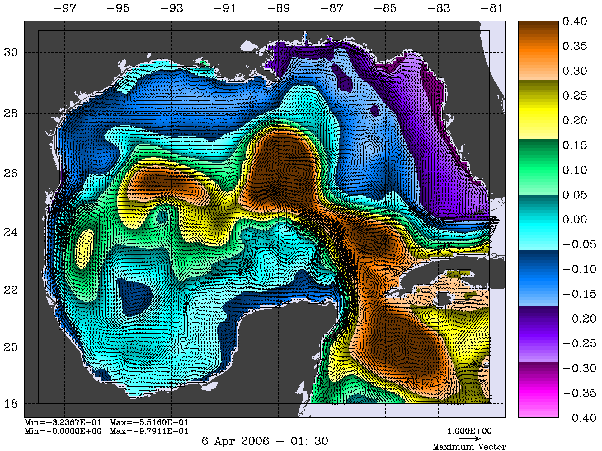
I updated the ROMS plotting package to write out the minimum and maximum values of the primary an secondary (overlay) fields. The above figure shows a snapshot of the free-surface and barotropic currents. Notice that the range of values for both fields are written on the bottom left corner of the plot for the primary (free-surface) and secondary overlay (barotropic currents) fields. The user can control the writing of the field statistics in the input scripts, see parameter WRTRANG: F PLTLOGO: logical switch Logo. F WRTHDR : logical switch to write out the plot header titles. T WRTBLAB: logical switch to write out the plot bottom title. T T WRTRANG: logical switch to write out data/overlay range values and CI. F WRTFNAM: logical switch to write out input primary filename. F WRTDATE: logical switch to write out current date. |
|||


