ROMS/TOMS Developers

Algorithms Update Web Log
« Previous Page

arango - August 4, 2006 @ 15:31
Background/Model Error Covariance Normalization- Comments (0)

In 4DVAR the background/model error covariance is modeled using a generalized diffusion operator. We use the approach of Weaver and Courtier (2001) to compute the correlation statistics. The normalization matrix is used to convert the covariance matrix into a correlation matrix. It insures that the diagonal elements of the background/model error covariance are equal to unity. The normalization matrix is spatially dependent and affected by the land/sea masking. Currently, there are two methods to compute these coefficients: exact (Nmethod=0) and randomization (Nmethod=1). The exact method is very expensive since the normalization coefficients are computed by perturbing each model grid cell with a delta function scaled by the area (2D) or volume (3D), and then convolving with the squared-root adjoint and tangent linear diffusion operators (ad_conv_2d.F, ad_conv_3d.F, tl_conv_2d.F, tl_conv_3d.F). The randomization (approximated) method is cheaper (Fisher and Courtier, 1995). The coefficients are initialized with random numbers having a uniform distribution (drawn from a normal distribution with zero mean and unit variance). Then, scaled by the inverse, squared-root cell area (2D) or volume (3D) and convolved with squared-root tangent linear diffusion operator. These normalization coefficients are computed in Utility/normalization.F. The correlation parameters are specified, for each state variable, in s4dvar.in. The horizontal and vertical decorrelation scales are Hdecay(:) and Vdecay(:), respectively. Check 4DVAR input script for more details. In realistic applications, it is highly recomended to do the vertical convolutions implicitly (IMPLICIT_VCONV). Otherwise, it will take too many iterations since the very different horizontal and vertical length scales.

Several plots are shown below for the normalization coefficients in the CHANNEL_NECK application. We are using a 10 km horizontal decorrelation scale and 10 m vertical decorrelation scale. This application is east-west periodic and has land/sea masking in the constriction. The normalization coefficents were computed using both exact and randomization methods. The number of iterations in the randomization method is set to Nrandom=50000 to achieve a statistical meaninfull population with approximately zero expectation mean and unit variance.

Normalization coefficients, 2D variable at RHO-points: Exact Method

Free-surface correlation normalization coefficient

Normalization coefficients, 2D variable at RHO-points: Randomization Method
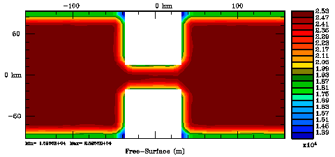
Free-surface correlation normalization coefficient, randomization

Normalization coefficients, 2D variable at U-points: Exact Method
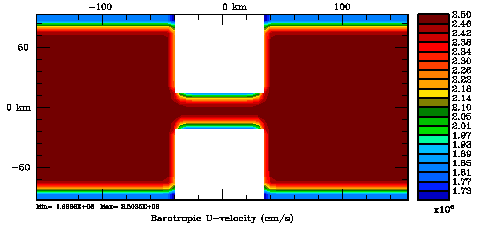
2D U-momentum correlation normalization coefficient

Normalization coefficients, 2D variable at U-points: Randomization Method
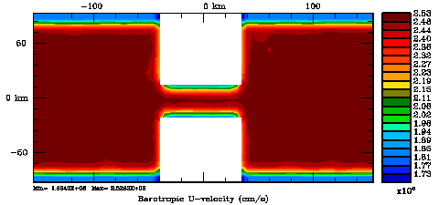
2D U-momentum correlation normalization coefficient, randomization

Normalization coefficients, 2D variable at V-points: Exact Method
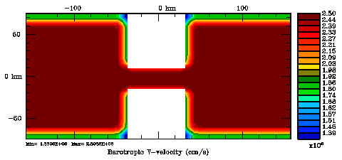
2D V-momentum correlation normalization coefficient

Normalization coefficients, 2D variable at V-points: Randomization Method

2D V-momentum correlation normalization coefficient, randomization

Normalization coefficients, 3D variable at RHO-points, surface level: Exact Method
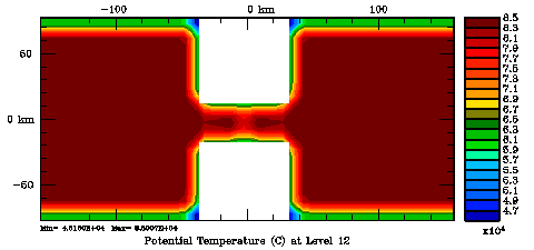
Tracers correlation normalization coefficient

Normalization coefficients, 3D variable at RHO-points, surface level: Randomization Method
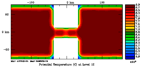
Tracers correlation normalization coefficient, randomization

Normalization coefficients, 3D variable at U-points, surface level: Exact Method
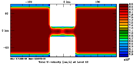
3D U-momentum correlation normalization coefficient

Normalization coefficients, 3D variable at U-points, surface level: Randomization Method
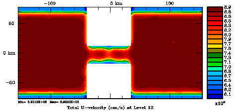
3D U-momentum correlation normalization coefficient, randomization

Normalization coefficients, 3D variable at V-points, surface level: Exact Method
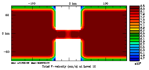
3D V-momentum correlation normalization coefficient

Normalization coefficients, 3D variable at V-points, surface level: Randomization Method
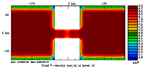
3D V-momentum correlation normalization coefficient, randomization


arango - August 4, 2006 @ 12:45
Updated Algorithms, Optimal Observations- Comments (0)

Updated version 3 algorithms to include optimal observations (OPT_OBSERVATIONS). Here is a summary of the changes:

  • Added new driver optobs_ocean.h.
  • Introduced new internal CPP option OBSERVATIONS in globaldefs.h to differentiate between 4DVAR related applications that require to process observations. This cleaned nicely several drivers. Several files were changed to achieve this.
  • Corrected extract_obs.F and ad_extract_obs.F to allow zero value depths, like when assimilating SST.
  • Corrected ad_conv_2d.F, ad_conv_3d.F, tl_conv_2d.F, tl_conv_3d.F, and normalization.F for periodic applications. Many thanks to Julia for helping me fix this bug. Now, the normalization factors used in the spatial convolution are truely periodic. Both exact and randomization methods are working correctly in periodic applications. Also the land/sea masking behavior between exact and randomization methods exhibits similar behavior: there is no increase in the normalization factors next to the mask. Non-periodic application were fine, except for the mask issue. Since we needed to change the spatial convolutions you need to recompute your normalization coefficients to ensure symmetry and unity correlations.
  • Renamed several CPP options in the tangent linear, representers, and adjoint models to the _NOT_YET to allow such options in the basic state (nonlinear model). These options included: BBL_MODEL, GLS_MIXING, MY25_MIXING, SEDIMENT, SSH_TIDES, and UV_TIDES.
  • Added the capability to write background and observation cost function, cost function norm, and optimality property into 4DVAR output NetCDF file (MODname). This only applies to IS4DVAR and S4DVAR options.
  • For the current updated file list .

arango - August 4, 2006 @ 12:45
Optimal Observations, New Driver- Comments (0)

I updated the codes to add a new driver to estimate optimal observations, OPT_OBSERVATIONS. Many thanks to Gordon for implementing this option. This driver is an enhanced adjoint sensitivity algorithm, but the tangent linear is used and initialized from the adjoint final record (initial time). As in the AD_SENSITIVITY case, the user need to define the chosen functional or index, J, in terms of the space and/or time integrals of the model state, S(zeta,u,v,T,…). Small changes, dS, in S will lead to changes dJ in J:

dJ = (dJ/dzeta) dzeta + (dJ/du) du + (dJ/dv) dv + (dJ/dt) dT ...

and

dJ/dS = transpose(R) S

where transpose(R) is the adjoint propagator. It implies that the sensitivity for ALL variables, parameters, and space-time points can be computed from a single integration of the adjoint model.

As in AD_SENSITIVITY, the user needs to provide the adjoint sensitivity scope arrays Rscope, Uscope, and Vscope in the GRID NetCDF file. It also needs to provide the basic state trajectory (nonlinear solution) that is used to linearize the adjoint and tangent linear models.


arango - July 26, 2006 @ 17:45
List of Updated files, Version 3.0- Comments (0)

We added a link that shows the files that have been modified in Version 3.0 at the Beta-Testers password protected link. This version was released on May 15, 2006. Corrected files will have newer dates. You just need to click on the listing button. This list is generated automatically every time that a new tar is uploaded.

For the current list .

arango - July 26, 2006 @ 17:30
Updated 4DVAR Algorithms, Version 3.0- Comments (0)

I updated several files to facilitate IOM’s multiple executable option and 4D-PSAS:

  • Renamed couple of CPP options for clarity: REPRESENTERS to WEAK_CONSTRAINT and IOM_MULTIPLE to IOM. The WEAK_CONSTRAINT option is now used for weak constraint data assimilation options W4DVAR and W4DPSAS. The IOM option is now used exclusively to interface with IOM’s GUI.
  • Corrected a bug in obs_cost.F that affected the step size computation used in the IS4DVAR and S4DVAR conjugate gradient algorithm. We were actually only using the last observation time survey. We need sum over all time surveys.
  • I added the optimalilty property test from Weaver et al. (2002). This is a good diagnostic to check the consistency between background and observation error covariance hypotheses (Chi-square test). The cost function value at the minimum, Jmin, is ideally equal to half the number of observations assimilated for a linear system. That is, Optimality=2*Jmin/Nobs. The theoretical value for this normalized quantity is Optimality=1. Therefore, the closer to unity the better. This is only available in the IS4DVAR driver. To check for this quantity grep for Optimality in the standard output file.
  • I fine tunned obs_read.F and obs_write.F to report rejected observations counters (land/sea masking and out of bounds observations). This required some changes to variable ObsScale. I am very happy about this change. It makes more sense now.