ROMS/TOMS Developers

Following Weaver and Courtier (2001), the vertical and horizontal correlations, C, for any state variable Φ are modeled using separated 1D and 2D diffusion equations:

where K_v and K_H are the vertical and horizontal diffusion coefficients (m²/s), assumed to be of order one. They are set to unity (isotropic correlations), if these coefficients are not found in ROMS/TOMS background/model standard deviation NetCDF file (STDname, variables K_v and K_h). The user can set K_v and K_h to the desired patterns to get anisotropic correlations. If we discretize the above diffusion operators using an explicit FTCS scheme, the stability limit is governed by:

In practice, we set γ < 1 to be below the stability threshold, (γ = 0.5). This stability parameter is set in 4DVAR input script. There are two variables: Vgamma and Hgamma for vertical and horizontal diffusion operators. In realistic applications, the vertical difussion needs to be solved implicitly (IMPLICIT_VCONV). Otherwise, the it will be very expensive since the vertical scales are much smaller. The implicit algorithm is unconditionally stable for any time-step, so we use the maximum thickness in the above equation instead of the minimum.

The parameters controlling the vertical and horizontal length-scales of the Gaussian correlation function are:

over a time interval 0 ≤ t ≤ T and

where M_v and M_H are the total number of vertical and horizontal integration steps. Notice that both values are forced to an even number since the squared-root diffusion operators are used to insure symmetry. The squared-root operator iterates only for half of the steps. For any given decorrelation length-scale, the number of integration steps are given by:

The vertical and horizontal decorrelation scales (m) are set in 4DVar input script variables Vdecay(:) and Hdecay(:) for each state variable.

ROMS/TOMS reports to standard output all the parameters associated with these diffusion operators. For example,

 5.0000E-01  Hgamma          Horizontal diffusion stability/accuracy factor.
 5.0000E-05  Vgamma          Vertical diffusion stability/accuracy factor.
  20000.000  Hdecay(isFsur)  Horizontal decorrelation scale (m), free-sruface.
  20000.000  Hdecay(isUbar)  Horizontal decorrelation scale (m), 2D U-momentum.
  20000.000  Hdecay(isVbar)  Horizontal decorrelation scale (m), 2D V-momentum.
  20000.000  Hdecay(isUvel)  Horizontal decorrelation scale (m), 3D U-momentum.
  20000.000  Hdecay(isVvel)  Horizontal decorrelation scale (m), 3D V-momentum.
  20000.000  Hdecay(idTvar)  Horizontal decorrelation scale (m), temp.
  20000.000  Hdecay(idTvar)  Horizontal decorrelation scale (m), salt.
      5.000  Vdecay(isUvel)  Vertical decorrelation scale (m), 3D U-momentum.
      5.000  Vdecay(isVvel)  Vertical decorrelation scale (m), 3D V-momentum.
      5.000  Vdecay(idTvar)  Vertical decorrelation scale (m), temp.
      5.000  Vdecay(idTvar)  Vertical decorrelation scale (m), salt.

 Minimum X-grid spacing, DXmin =  5.26835784E+00 km
 Maximum X-grid spacing, DXmax =  5.58390264E+00 km
 Minimum Y-grid spacing, DYmin =  5.05224079E+00 km
 Maximum Y-grid spacing, DYmax =  5.35460591E+00 km
 Minimum Z-grid spacing, DZmin =  1.33333333E-01 m
 Maximum Z-grid spacing, DZmax =  2.86550363E+02 m

 Minimum barotropic Courant Number =  2.99123135E-02
 Maximum barotropic Courant Number =  8.17259140E-01
 Maximum Coriolis   Courant Number =  3.43845829E-02

 Horizontal convolution, NHsteps, DTsizeH =    64  3.19064213E+06 s  zeta
 Horizontal convolution, NHsteps, DTsizeH =    64  3.19064213E+06 s  ubar
 Horizontal convolution, NHsteps, DTsizeH =    64  3.19064213E+06 s  vbar
 Horizontal convolution, NHsteps, DTsizeH =    64  3.19064213E+06 s  u
 Horizontal convolution, NHsteps, DTsizeH =    64  3.19064213E+06 s  v
 Horizontal convolution, NHsteps, DTsizeH =    64  3.19064213E+06 s  temp
 Horizontal convolution, NHsteps, DTsizeH =    64  3.19064213E+06 s  salt

 Vertical   convolution, NVsteps, DTsizeV =     6  2.05277776E+00 s  u
 Vertical   convolution, NVsteps, DTsizeV =     6  2.05277776E+00 s  v
 Vertical   convolution, NVsteps, DTsizeV =     6  2.05277776E+00 s  temp
 Vertical   convolution, NVsteps, DTsizeV =     6  2.05277776E+00 s  salt

It is recommended to reduce the Vgamma parameter until a value of M_v is around six for vertical diffusion accuracy.

The incremental, strong contraint 4DVAR (IS4DVAR) approximated approach was proposed by Courtier et al. (1994) to reduce the computational cost and facilitate better preconditioning. We follow the algorithm proposed by Weaver et al (2002) that defines the increment to the difference from previous reference state.

Let x^k denote the state vector on the k-th outer loop such that δx^k is the increment difference from the previous state

where x^{k -1} is the current estimate of the ocean state. It is equal to the background state for the first minimization (x⁰ = x_b, δx¹ = 0). The cost function on the k-th loop can be written as

where d^{k – 1} = x_o – Hx^{k – 1} is the innovation vector, x_o is the observation vector, x_b is the background state, H is a linear approximation of the observation operator H, and B and O are the background and observation error covariance matrices. Let’s introduce a new minimization variable δv, such that:

It is more convenient to work in terms of δv (minimization space: v-space). The conditioning of the J_b in v-space is optimal since it’s Hessian, ∂²J_b/∂v², yields the identity matrix. The gradient of J in v-space, denoted ∇_vJ, is given by:

where B = B^T/2B^1/2 and B^T/2 denotes (B^1/2)^T, and ∇_xJ_o is the gradient of J_o in model space (x-space) which is computed using the adjoint model and given by:

Following Weaver and Courtier (2001), the background-error covariance matrix can be factored as:

where S is a diagonal matrix of background-error standard deviations, C is a symetric matrix of background-error correlations which can be factorized as C = C^1/2C^T/2, G is the normalization matrix which ensures that the diagonal elements of C are equal to unity, L is a 3D self-adjoint filtering operator, and W is the grid cell area (2D fields) or volume (3D fields).

• Corrected few bugs in the optimal observation driver, OPT_OBSERVATIONS. Many thanks to Julia for help me tracking these bugs. This driver seems to be working well and can be used in adaptive sampling to help designing observational networks.
• Commented out the warning message in opencdf.F when the global attribute is missing in input NetCDF files.
• Added a new set-up for the Shallow Water 2006 Experiment in the Mid-Atlantic Bight. This application has a coarse and finer grid: SW06_COARSE and SW06_FINE.
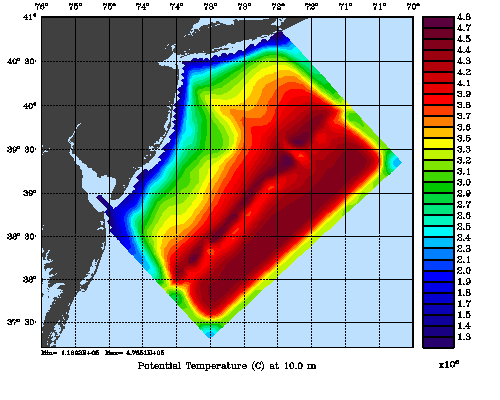
• The 4DVAR background covariance normalization coefficients for tracers is shown below for SW06_COARSE:

These are computed using the exact method for a horizontal and vertical decorrelation scales of 20 km and 20 m, respectively. This implies that the horizontal convolution for these length scales requires 64 iterations of the horizontal diffusion and only 2 iterations of the implicit vertical diffusion. The implicit diffusion is unconditionally stable so we can take very large time-steps, even if the minimum thickness is just 1.3 m. In this application we are using a value of Hgamma=0.5 and Vgamma=0.05. Hgamma and Vgamma are the horizontal and vertical stability and accuaracy factors used to scale the time-step of the convolution operator below its theorethical limit. The value of Vgamma is forced to be small in the implicit computation to insure at least two iterations. Also notice that the number of iterations, NHsteps and NVsteps, are always forced to be even since only half of the steps are iterated in the squared-root tangent linear and adjoint diffusion operators. Please always check these values written to standard output before using the 4DVAR algorithms.

 Minimum X-grid spacing, DXmin =  5.26835784E+00 km
 Maximum X-grid spacing, DXmax =  5.58390264E+00 km
 Minimum Y-grid spacing, DYmin =  5.05224079E+00 km
 Maximum Y-grid spacing, DYmax =  5.35460591E+00 km
 Minimum Z-grid spacing, DZmin =  1.33333333E-01 m
 Maximum Z-grid spacing, DZmax =  2.86550363E+02 m

 Horizontal convolution, NHsteps, DTsizeH =    64  3.19064213E+06 s  zeta
 Horizontal convolution, NHsteps, DTsizeH =    64  3.19064213E+06 s  ubar
 Horizontal convolution, NHsteps, DTsizeH =    64  3.19064213E+06 s  vbar
 Horizontal convolution, NHsteps, DTsizeH =    64  3.19064213E+06 s  u
 Horizontal convolution, NHsteps, DTsizeH =    64  3.19064213E+06 s  v
 Horizontal convolution, NHsteps, DTsizeH =    64  3.19064213E+06 s  temp
 Horizontal convolution, NHsteps, DTsizeH =    64  3.19064213E+06 s  salt

 Vertical   convolution, NVsteps, DTsizeV =     2  2.05277776E+03 s  u
 Vertical   convolution, NVsteps, DTsizeV =     2  2.05277776E+03 s  v
 Vertical   convolution, NVsteps, DTsizeV =     2  2.05277776E+03 s  temp
 Vertical   convolution, NVsteps, DTsizeV =     2  2.05277776E+03 s  salt

Below is the profiling numbers for East Australia Current Application (EAC_4), 64x80x30 grid points, on 4-CPUs with 1×4 partition in my Linux Box:

Linux 2.6.12-15mdksmp #1 SMP Mon Jan 9 23:35:18 MST 2006 x86_64 Dual Core AMD Opteron(tm) Processor 265

The nonlinear model is run for 800 time-steps as standalone driver with the same CPP options as the tangent linear, adjoint and representer models. The vertical mixing parameterization is set to a constant for all models.

Nonlinear model elapsed time profile:

  Initialization ...................................         4.587  ( 0.7179 %)
  Reading of input data ............................         3.979  ( 0.6226 %)
  Processing of input data .........................         7.522  ( 1.1772 %)
  Computation of vertical boundary conditions ......         0.625  ( 0.0978 %)
  Computation of global information integrals ......         8.183  ( 1.2807 %)
  Writing of output data ...........................         7.926  ( 1.2404 %)
  Model 2D kernel ..................................       359.438  (56.2512 %)
  2D/3D coupling, vertical metrics .................        12.438  ( 1.9465 %)
  Omega vertical velocity ..........................        16.498  ( 2.5818 %)
  Equation of state for seawater ...................        13.606  ( 2.1292 %)
  3D equations right-side terms ....................        23.653  ( 3.7016 %)
  3D equations predictor step ......................        57.813  ( 9.0476 %)
  Pressure gradient ................................        22.302  ( 3.4901 %)
  Harmonic stress tensor, S-surfaces ...............         9.827  ( 1.5379 %)
  Corrector time-step for 3D momentum ..............        37.238  ( 5.8277 %)
  Corrector time-step for tracers ..................        37.273  ( 5.8331 %)
                                              Total:       622.907   97.4834

 Nonlinear model message Passage profile:

  Message Passage: 2D halo exchanges ...............       140.839  (22.0409 %)
  Message Passage: 3D halo exchanges ...............        29.981  ( 4.6920 %)
  Message Passage: 4D halo exchanges ...............        11.629  ( 1.8199 %)
  Message Passage: data broadcast ..................         6.781  ( 1.0612 %)
  Message Passage: data reduction ..................         1.470  ( 0.2301 %)
  Message Passage: data gathering ..................         2.517  ( 0.3939 %)
  Message Passage: data scattering..................         3.362  ( 0.5262 %)
                                              Total:       196.579   30.7641

 All pecentages are with respect to total time =           638.988

The tangent linear and adjoint models are run together using the SANITY_CHECK driver, so the total elapsed time accounts for both models.

 Tangent linear model elapsed time profile:

  Initialization ...................................        14.835  ( 0.4350 %)
  Reading of input data ............................       173.861  ( 5.0979 %)
  Processing of input data .........................        95.638  ( 2.8043 %)
  Computation of vertical boundary conditions ......         0.875  ( 0.0256 %)
  Computation of global information integrals ......         8.092  ( 0.2373 %)
  Writing of output data ...........................         4.161  ( 0.1220 %)
  Model 2D kernel ..................................       828.082  (24.2810 %)
  2D/3D coupling, vertical metrics .................        18.079  ( 0.5301 %)
  Omega vertical velocity ..........................        31.976  ( 0.9376 %)
  Equation of state for seawater ...................        27.216  ( 0.7980 %)
  3D equations right-side terms ....................        44.738  ( 1.3118 %)
  3D equations predictor step ......................        98.420  ( 2.8859 %)
  Pressure gradient ................................        44.543  ( 1.3061 %)
  Harmonic stress tensor, S-surfaces ...............        13.495  ( 0.3957 %)
  Corrector time-step for 3D momentum ..............        74.287  ( 2.1782 %)
  Corrector time-step for tracers ..................        72.838  ( 2.1358 %)
                                              Total:      1551.133   45.4823

Tangent linear model message Passage profile:

  Message Passage: 2D halo exchanges ...............       223.804  ( 6.5624 %)
  Message Passage: 3D halo exchanges ...............        55.990  ( 1.6417 %)
  Message Passage: 4D halo exchanges ...............         7.083  ( 0.2077 %)
  Message Passage: data broadcast ..................        10.551  ( 0.3094 %)
  Message Passage: data reduction ..................         1.248  ( 0.0366 %)
  Message Passage: data gathering ..................         1.241  ( 0.0364 %)
  Message Passage: data scattering..................       132.319  ( 3.8799 %)
  Message Passage: point data gathering ............         0.004  ( 0.0001 %)
                                              Total:       432.240   12.6741

 Adjoint model elapsed time profile:

  Initialization ...................................         6.466  ( 0.1896 %)
  Reading of input data ............................        47.553  ( 1.3944 %)
  Processing of input data .........................        93.203  ( 2.7329 %)
  Computation of vertical boundary conditions ......         1.597  ( 0.0468 %)
  Computation of global information integrals ......         8.488  ( 0.2489 %)
  Writing of output data ...........................         5.610  ( 0.1645 %)
  Model 2D kernel ..................................      1008.202  (29.5625 %)
  2D/3D coupling, vertical metrics .................        31.938  ( 0.9365 %)
  Omega vertical velocity ..........................        45.539  ( 1.3353 %)
  Equation of state for seawater ...................        42.038  ( 1.2326 %)
  3D equations right-side terms ....................        55.763  ( 1.6351 %)
  3D equations predictor step ......................       138.419  ( 4.0587 %)
  Pressure gradient ................................        68.866  ( 2.0193 %)
  Harmonic stress tensor, S-surfaces ...............        20.567  ( 0.6031 %)
  Corrector time-step for 3D momentum ..............        80.219  ( 2.3522 %)
  Corrector time-step for tracers ..................        98.440  ( 2.8865 %)
                                              Total:      1752.908   51.3987

 Adjoint model message Passage profile:

  Message Passage: 2D halo exchanges ...............       255.896  ( 7.5034 %)
  Message Passage: 3D halo exchanges ...............        71.025  ( 2.0826 %)
  Message Passage: 4D halo exchanges ...............        15.459  ( 0.4533 %)
  Message Passage: data broadcast ..................         8.647  ( 0.2535 %)
  Message Passage: data reduction ..................         1.842  ( 0.0540 %)
  Message Passage: data gathering ..................         1.750  ( 0.0513 %)
  Message Passage: data scattering..................        42.078  ( 1.2338 %)
                                              Total:       396.695   11.6319

 All pecentages are with respect to total time =          3410.412

The representer tangent linear model is run as a separated driver using TLM_DRIVER.

 Representer model elapsed time profile:

  Initialization ...................................         4.597  ( 0.2799 %)
  Reading of input data ............................        38.600  ( 2.3505 %)
  Processing of input data .........................        95.962  ( 5.8436 %)
  Computation of vertical boundary conditions ......         1.309  ( 0.0797 %)
  Computation of global information integrals ......         8.371  ( 0.5098 %)
  Writing of output data ...........................         4.301  ( 0.2619 %)
  Model 2D kernel ..................................      1007.191  (61.3323 %)
  2D/3D coupling, vertical metrics .................        18.687  ( 1.1379 %)
  Omega vertical velocity ..........................        32.856  ( 2.0007 %)
  Equation of state for seawater ...................        33.136  ( 2.0178 %)
  3D equations right-side terms ....................        49.279  ( 3.0008 %)
  3D equations predictor step ......................       101.300  ( 6.1686 %)
  Pressure gradient ................................        46.778  ( 2.8485 %)
  Harmonic stress tensor, S-surfaces ...............        14.770  ( 0.8994 %)
  Corrector time-step for 3D momentum ..............        76.202  ( 4.6403 %)
  Corrector time-step for tracers ..................        75.721  ( 4.6110 %)
                                              Total:      1609.061   97.9828

 Representer model message Passage profile:

  Message Passage: 2D halo exchanges ...............       241.656  (14.7155 %)
  Message Passage: 3D halo exchanges ...............        58.278  ( 3.5488 %)
  Message Passage: 4D halo exchanges ...............        13.696  ( 0.8340 %)
  Message Passage: data broadcast ..................         3.486  ( 0.2123 %)
  Message Passage: data reduction ..................         1.426  ( 0.0868 %)
  Message Passage: data scattering..................        33.392  ( 2.0334 %)
                                              Total:       351.935   21.4308

 All pecentages are with respect to total time =          1642.187

If we take the timings for the kernel and ignore the rest and normalize with respect the nonlinear model we get:

   
  Tangent linear model:    1551/622 = 2.49
  Representer model        1609/622 = 2.59
  Adjoint model:           1752/622 = 2.82
 

That is, the tangent linear is model is approximately 2.5 times expensier than the nonlinear model. The representer model is about 2.6 times expensier than the nonlinear model and around 3-percent expensier that the tangent linear model. The adjoint model is about 2.8 times expensier than the nolinear model and around 12-percent expensier than the tangent linear model.

Two of my biological ROMS associates came to me with a problem. We tracked it down to mod_average.F, which should have this code:

        DO itrc=1,NT(ng)
          DO k=1,N(ng)
            DO i=Imin,Imax
              AVERAGE(ng) % avgt(i,j,k,itrc) = IniVal
            END DO
            END DO
          END DO
        END DO
#  ifdef AVERAGES_QUADRATIC
        DO itrc=1,NAT
          DO k=1,N(ng)
            DO i=Imin,Imax
              AVERAGE(ng) % avgTT(i,j,k,itrc) = IniVal
              AVERAGE(ng) % avgUT(i,j,k,itrc) = IniVal
              AVERAGE(ng) % avgVT(i,j,k,itrc) = IniVal
            END DO 
          END DO
        END DO
#  endif

It was failing in the NetCDF write of avgt(:,:.:,3) (Nitrate). When ROMS dies in this situation, it says it has trouble in the write from wrt_avg of Nitrate, but it doesn’t give the NetCDF error message. I would like to see us not only check for errors, but print out the NetCDF error from the error code. I have a f90 code which uses this function:

  subroutine check(status)
    integer, intent(in) :: status
    if (status /= nf90_noerr) then
      print *, nf90_strerror(status)
      call exit(1)
    endif
  end subroutine check

It is used like this:

   call check(nf90_inq_varid(fileID, 'vals_nod_var', varid))
   call check(nf90_put_var(fileID, varid, size, &
          start = (/ 1, 1, 1 /), count = (/ nnodes, 1, 1 /) ))