ROMS/TOMS Developers

Algorithms Update Web Log
« Previous PageNext Page »

arango - August 11, 2006 @ 21:38
Fixed Optimal Observations Driver, Version 3.0- Comments (0)

  • Corrected few bugs in the optimal observation driver, OPT_OBSERVATIONS. Many thanks to Julia for help me tracking these bugs. This driver seems to be working well and can be used in adaptive sampling to help designing observational networks.
  • Commented out the warning message in opencdf.F when the global attribute is missing in input NetCDF files.
  • Added a new set-up for the Shallow Water 2006 Experiment in the Mid-Atlantic Bight. This application has a coarse and finer grid: SW06_COARSE and SW06_FINE.
  • The 4DVAR background covariance normalization coefficients for tracers is shown below for SW06_COARSE:
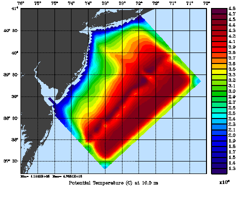
SW06c background covariance normalization coefficient, exact

These are computed using the exact method for a horizontal and vertical decorrelation scales of 20 km and 20 m, respectively. This implies that the horizontal convolution for these length scales requires 64 iterations of the horizontal diffusion and only 2 iterations of the implicit vertical diffusion. The implicit diffusion is unconditionally stable so we can take very large time-steps, even if the minimum thickness is just 1.3 m. In this application we are using a value of Hgamma=0.5 and Vgamma=0.05. Hgamma and Vgamma are the horizontal and vertical stability and accuaracy factors used to scale the time-step of the convolution operator below its theorethical limit. The value of Vgamma is forced to be small in the implicit computation to insure at least two iterations. Also notice that the number of iterations, NHsteps and NVsteps, are always forced to be even since only half of the steps are iterated in the squared-root tangent linear and adjoint diffusion operators. Please always check these values written to standard output before using the 4DVAR algorithms.

 Minimum X-grid spacing, DXmin =  5.26835784E+00 km
 Maximum X-grid spacing, DXmax =  5.58390264E+00 km
 Minimum Y-grid spacing, DYmin =  5.05224079E+00 km
 Maximum Y-grid spacing, DYmax =  5.35460591E+00 km
 Minimum Z-grid spacing, DZmin =  1.33333333E-01 m
 Maximum Z-grid spacing, DZmax =  2.86550363E+02 m

 Horizontal convolution, NHsteps, DTsizeH =    64  3.19064213E+06 s  zeta
 Horizontal convolution, NHsteps, DTsizeH =    64  3.19064213E+06 s  ubar
 Horizontal convolution, NHsteps, DTsizeH =    64  3.19064213E+06 s  vbar
 Horizontal convolution, NHsteps, DTsizeH =    64  3.19064213E+06 s  u
 Horizontal convolution, NHsteps, DTsizeH =    64  3.19064213E+06 s  v
 Horizontal convolution, NHsteps, DTsizeH =    64  3.19064213E+06 s  temp
 Horizontal convolution, NHsteps, DTsizeH =    64  3.19064213E+06 s  salt

 Vertical   convolution, NVsteps, DTsizeV =     2  2.05277776E+03 s  u
 Vertical   convolution, NVsteps, DTsizeV =     2  2.05277776E+03 s  v
 Vertical   convolution, NVsteps, DTsizeV =     2  2.05277776E+03 s  temp
 Vertical   convolution, NVsteps, DTsizeV =     2  2.05277776E+03 s  salt

arango - August 9, 2006 @ 16:43
Profiling Nonlinear, Tangent Linear and Adjoint Models- Comments (0)

Below is the profiling numbers for East Australia Current Application (EAC_4), 64x80x30 grid points, on 4-CPUs with 1×4 partition in my Linux Box:

Linux 2.6.12-15mdksmp #1 SMP Mon Jan 9 23:35:18 MST 2006 x86_64 Dual Core AMD Opteron(tm) Processor 265

The nonlinear model is run for 800 time-steps as standalone driver with the same CPP options as the tangent linear, adjoint and representer models. The vertical mixing parameterization is set to a constant for all models.

Nonlinear model elapsed time profile:

  Initialization ...................................         4.587  ( 0.7179 %)
  Reading of input data ............................         3.979  ( 0.6226 %)
  Processing of input data .........................         7.522  ( 1.1772 %)
  Computation of vertical boundary conditions ......         0.625  ( 0.0978 %)
  Computation of global information integrals ......         8.183  ( 1.2807 %)
  Writing of output data ...........................         7.926  ( 1.2404 %)
  Model 2D kernel ..................................       359.438  (56.2512 %)
  2D/3D coupling, vertical metrics .................        12.438  ( 1.9465 %)
  Omega vertical velocity ..........................        16.498  ( 2.5818 %)
  Equation of state for seawater ...................        13.606  ( 2.1292 %)
  3D equations right-side terms ....................        23.653  ( 3.7016 %)
  3D equations predictor step ......................        57.813  ( 9.0476 %)
  Pressure gradient ................................        22.302  ( 3.4901 %)
  Harmonic stress tensor, S-surfaces ...............         9.827  ( 1.5379 %)
  Corrector time-step for 3D momentum ..............        37.238  ( 5.8277 %)
  Corrector time-step for tracers ..................        37.273  ( 5.8331 %)
                                              Total:       622.907   97.4834

 Nonlinear model message Passage profile:

  Message Passage: 2D halo exchanges ...............       140.839  (22.0409 %)
  Message Passage: 3D halo exchanges ...............        29.981  ( 4.6920 %)
  Message Passage: 4D halo exchanges ...............        11.629  ( 1.8199 %)
  Message Passage: data broadcast ..................         6.781  ( 1.0612 %)
  Message Passage: data reduction ..................         1.470  ( 0.2301 %)
  Message Passage: data gathering ..................         2.517  ( 0.3939 %)
  Message Passage: data scattering..................         3.362  ( 0.5262 %)
                                              Total:       196.579   30.7641

 All pecentages are with respect to total time =           638.988

The tangent linear and adjoint models are run together using the SANITY_CHECK driver, so the total elapsed time accounts for both models.

 Tangent linear model elapsed time profile:

  Initialization ...................................        14.835  ( 0.4350 %)
  Reading of input data ............................       173.861  ( 5.0979 %)
  Processing of input data .........................        95.638  ( 2.8043 %)
  Computation of vertical boundary conditions ......         0.875  ( 0.0256 %)
  Computation of global information integrals ......         8.092  ( 0.2373 %)
  Writing of output data ...........................         4.161  ( 0.1220 %)
  Model 2D kernel ..................................       828.082  (24.2810 %)
  2D/3D coupling, vertical metrics .................        18.079  ( 0.5301 %)
  Omega vertical velocity ..........................        31.976  ( 0.9376 %)
  Equation of state for seawater ...................        27.216  ( 0.7980 %)
  3D equations right-side terms ....................        44.738  ( 1.3118 %)
  3D equations predictor step ......................        98.420  ( 2.8859 %)
  Pressure gradient ................................        44.543  ( 1.3061 %)
  Harmonic stress tensor, S-surfaces ...............        13.495  ( 0.3957 %)
  Corrector time-step for 3D momentum ..............        74.287  ( 2.1782 %)
  Corrector time-step for tracers ..................        72.838  ( 2.1358 %)
                                              Total:      1551.133   45.4823

Tangent linear model message Passage profile:

  Message Passage: 2D halo exchanges ...............       223.804  ( 6.5624 %)
  Message Passage: 3D halo exchanges ...............        55.990  ( 1.6417 %)
  Message Passage: 4D halo exchanges ...............         7.083  ( 0.2077 %)
  Message Passage: data broadcast ..................        10.551  ( 0.3094 %)
  Message Passage: data reduction ..................         1.248  ( 0.0366 %)
  Message Passage: data gathering ..................         1.241  ( 0.0364 %)
  Message Passage: data scattering..................       132.319  ( 3.8799 %)
  Message Passage: point data gathering ............         0.004  ( 0.0001 %)
                                              Total:       432.240   12.6741

 Adjoint model elapsed time profile:

  Initialization ...................................         6.466  ( 0.1896 %)
  Reading of input data ............................        47.553  ( 1.3944 %)
  Processing of input data .........................        93.203  ( 2.7329 %)
  Computation of vertical boundary conditions ......         1.597  ( 0.0468 %)
  Computation of global information integrals ......         8.488  ( 0.2489 %)
  Writing of output data ...........................         5.610  ( 0.1645 %)
  Model 2D kernel ..................................      1008.202  (29.5625 %)
  2D/3D coupling, vertical metrics .................        31.938  ( 0.9365 %)
  Omega vertical velocity ..........................        45.539  ( 1.3353 %)
  Equation of state for seawater ...................        42.038  ( 1.2326 %)
  3D equations right-side terms ....................        55.763  ( 1.6351 %)
  3D equations predictor step ......................       138.419  ( 4.0587 %)
  Pressure gradient ................................        68.866  ( 2.0193 %)
  Harmonic stress tensor, S-surfaces ...............        20.567  ( 0.6031 %)
  Corrector time-step for 3D momentum ..............        80.219  ( 2.3522 %)
  Corrector time-step for tracers ..................        98.440  ( 2.8865 %)
                                              Total:      1752.908   51.3987

 Adjoint model message Passage profile:

  Message Passage: 2D halo exchanges ...............       255.896  ( 7.5034 %)
  Message Passage: 3D halo exchanges ...............        71.025  ( 2.0826 %)
  Message Passage: 4D halo exchanges ...............        15.459  ( 0.4533 %)
  Message Passage: data broadcast ..................         8.647  ( 0.2535 %)
  Message Passage: data reduction ..................         1.842  ( 0.0540 %)
  Message Passage: data gathering ..................         1.750  ( 0.0513 %)
  Message Passage: data scattering..................        42.078  ( 1.2338 %)
                                              Total:       396.695   11.6319

 All pecentages are with respect to total time =          3410.412

The representer tangent linear model is run as a separated driver using TLM_DRIVER.

 Representer model elapsed time profile:

  Initialization ...................................         4.597  ( 0.2799 %)
  Reading of input data ............................        38.600  ( 2.3505 %)
  Processing of input data .........................        95.962  ( 5.8436 %)
  Computation of vertical boundary conditions ......         1.309  ( 0.0797 %)
  Computation of global information integrals ......         8.371  ( 0.5098 %)
  Writing of output data ...........................         4.301  ( 0.2619 %)
  Model 2D kernel ..................................      1007.191  (61.3323 %)
  2D/3D coupling, vertical metrics .................        18.687  ( 1.1379 %)
  Omega vertical velocity ..........................        32.856  ( 2.0007 %)
  Equation of state for seawater ...................        33.136  ( 2.0178 %)
  3D equations right-side terms ....................        49.279  ( 3.0008 %)
  3D equations predictor step ......................       101.300  ( 6.1686 %)
  Pressure gradient ................................        46.778  ( 2.8485 %)
  Harmonic stress tensor, S-surfaces ...............        14.770  ( 0.8994 %)
  Corrector time-step for 3D momentum ..............        76.202  ( 4.6403 %)
  Corrector time-step for tracers ..................        75.721  ( 4.6110 %)
                                              Total:      1609.061   97.9828

 Representer model message Passage profile:

  Message Passage: 2D halo exchanges ...............       241.656  (14.7155 %)
  Message Passage: 3D halo exchanges ...............        58.278  ( 3.5488 %)
  Message Passage: 4D halo exchanges ...............        13.696  ( 0.8340 %)
  Message Passage: data broadcast ..................         3.486  ( 0.2123 %)
  Message Passage: data reduction ..................         1.426  ( 0.0868 %)
  Message Passage: data scattering..................        33.392  ( 2.0334 %)
                                              Total:       351.935   21.4308

 All pecentages are with respect to total time =          1642.187

If we take the timings for the kernel and ignore the rest and normalize with respect the nonlinear model we get:

   
  Tangent linear model:    1551/622 = 2.49
  Representer model        1609/622 = 2.59
  Adjoint model:           1752/622 = 2.82
 

That is, the tangent linear is model is approximately 2.5 times expensier than the nonlinear model. The representer model is about 2.6 times expensier than the nonlinear model and around 3-percent expensier that the tangent linear model. The adjoint model is about 2.8 times expensier than the nolinear model and around 12-percent expensier than the tangent linear model.


kate - August 9, 2006 @ 14:07
Initialization and I/O- Comments (1)

Two of my biological ROMS associates came to me with a problem. We tracked it down to mod_average.F, which should have this code:

        DO itrc=1,NT(ng)
          DO k=1,N(ng)
            DO i=Imin,Imax
              AVERAGE(ng) % avgt(i,j,k,itrc) = IniVal
            END DO
            END DO
          END DO
        END DO
#  ifdef AVERAGES_QUADRATIC
        DO itrc=1,NAT
          DO k=1,N(ng)
            DO i=Imin,Imax
              AVERAGE(ng) % avgTT(i,j,k,itrc) = IniVal
              AVERAGE(ng) % avgUT(i,j,k,itrc) = IniVal
              AVERAGE(ng) % avgVT(i,j,k,itrc) = IniVal
            END DO 
          END DO
        END DO
#  endif

It was failing in the NetCDF write of avgt(:,:.:,3) (Nitrate). When ROMS dies in this situation, it says it has trouble in the write from wrt_avg of Nitrate, but it doesn’t give the NetCDF error message. I would like to see us not only check for errors, but print out the NetCDF error from the error code. I have a f90 code which uses this function:

  subroutine check(status)
    integer, intent(in) :: status
    if (status /= nf90_noerr) then
      print *, nf90_strerror(status)
      call exit(1)
    endif
  end subroutine check

It is used like this:

   call check(nf90_inq_varid(fileID, 'vals_nod_var', varid))
   call check(nf90_put_var(fileID, varid, size, &
          start = (/ 1, 1, 1 /), count = (/ nnodes, 1, 1 /) ))

arango - August 4, 2006 @ 15:31
Background/Model Error Covariance Normalization- Comments (0)

In 4DVAR the background/model error covariance is modeled using a generalized diffusion operator. We use the approach of Weaver and Courtier (2001) to compute the correlation statistics. The normalization matrix is used to convert the covariance matrix into a correlation matrix. It insures that the diagonal elements of the background/model error covariance are equal to unity. The normalization matrix is spatially dependent and affected by the land/sea masking. Currently, there are two methods to compute these coefficients: exact (Nmethod=0) and randomization (Nmethod=1). The exact method is very expensive since the normalization coefficients are computed by perturbing each model grid cell with a delta function scaled by the area (2D) or volume (3D), and then convolving with the squared-root adjoint and tangent linear diffusion operators (ad_conv_2d.F, ad_conv_3d.F, tl_conv_2d.F, tl_conv_3d.F). The randomization (approximated) method is cheaper (Fisher and Courtier, 1995). The coefficients are initialized with random numbers having a uniform distribution (drawn from a normal distribution with zero mean and unit variance). Then, scaled by the inverse, squared-root cell area (2D) or volume (3D) and convolved with squared-root tangent linear diffusion operator. These normalization coefficients are computed in Utility/normalization.F. The correlation parameters are specified, for each state variable, in s4dvar.in. The horizontal and vertical decorrelation scales are Hdecay(:) and Vdecay(:), respectively. Check 4DVAR input script for more details. In realistic applications, it is highly recomended to do the vertical convolutions implicitly (IMPLICIT_VCONV). Otherwise, it will take too many iterations since the very different horizontal and vertical length scales.

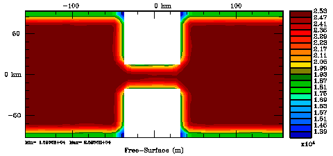
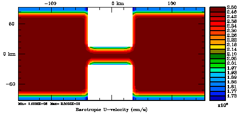
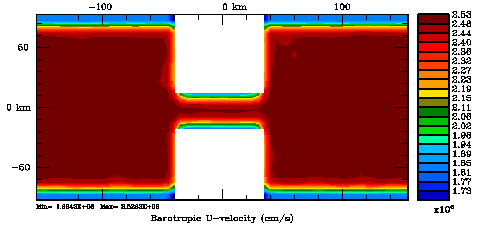
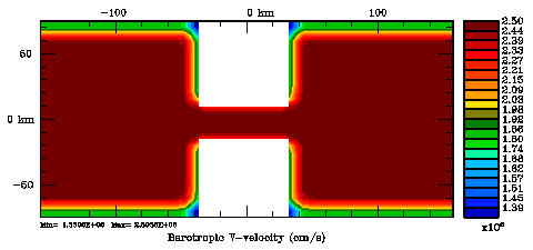
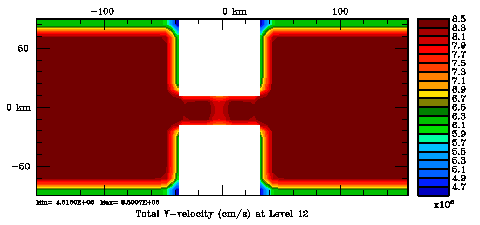
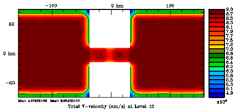
Several plots are shown below for the normalization coefficients in the CHANNEL_NECK application. We are using a 10 km horizontal decorrelation scale and 10 m vertical decorrelation scale. This application is east-west periodic and has land/sea masking in the constriction. The normalization coefficents were computed using both exact and randomization methods. The number of iterations in the randomization method is set to Nrandom=50000 to achieve a statistical meaninfull population with approximately zero expectation mean and unit variance.

Normalization coefficients, 2D variable at RHO-points: Exact Method

Free-surface correlation normalization coefficient

Normalization coefficients, 2D variable at RHO-points: Randomization Method

Free-surface correlation normalization coefficient, randomization

Normalization coefficients, 2D variable at U-points: Exact Method

2D U-momentum correlation normalization coefficient

Normalization coefficients, 2D variable at U-points: Randomization Method

2D U-momentum correlation normalization coefficient, randomization

Normalization coefficients, 2D variable at V-points: Exact Method

2D V-momentum correlation normalization coefficient

Normalization coefficients, 2D variable at V-points: Randomization Method

2D V-momentum correlation normalization coefficient, randomization

Normalization coefficients, 3D variable at RHO-points, surface level: Exact Method

Tracers correlation normalization coefficient

Normalization coefficients, 3D variable at RHO-points, surface level: Randomization Method

Tracers correlation normalization coefficient, randomization

Normalization coefficients, 3D variable at U-points, surface level: Exact Method

3D U-momentum correlation normalization coefficient

Normalization coefficients, 3D variable at U-points, surface level: Randomization Method

3D U-momentum correlation normalization coefficient, randomization

Normalization coefficients, 3D variable at V-points, surface level: Exact Method

3D V-momentum correlation normalization coefficient

Normalization coefficients, 3D variable at V-points, surface level: Randomization Method

3D V-momentum correlation normalization coefficient, randomization


arango - August 4, 2006 @ 12:45
Updated Algorithms, Optimal Observations- Comments (0)

Updated version 3 algorithms to include optimal observations (OPT_OBSERVATIONS). Here is a summary of the changes:

  • Added new driver optobs_ocean.h.
  • Introduced new internal CPP option OBSERVATIONS in globaldefs.h to differentiate between 4DVAR related applications that require to process observations. This cleaned nicely several drivers. Several files were changed to achieve this.
  • Corrected extract_obs.F and ad_extract_obs.F to allow zero value depths, like when assimilating SST.
  • Corrected ad_conv_2d.F, ad_conv_3d.F, tl_conv_2d.F, tl_conv_3d.F, and normalization.F for periodic applications. Many thanks to Julia for helping me fix this bug. Now, the normalization factors used in the spatial convolution are truely periodic. Both exact and randomization methods are working correctly in periodic applications. Also the land/sea masking behavior between exact and randomization methods exhibits similar behavior: there is no increase in the normalization factors next to the mask. Non-periodic application were fine, except for the mask issue. Since we needed to change the spatial convolutions you need to recompute your normalization coefficients to ensure symmetry and unity correlations.
  • Renamed several CPP options in the tangent linear, representers, and adjoint models to the _NOT_YET to allow such options in the basic state (nonlinear model). These options included: BBL_MODEL, GLS_MIXING, MY25_MIXING, SEDIMENT, SSH_TIDES, and UV_TIDES.
  • Added the capability to write background and observation cost function, cost function norm, and optimality property into 4DVAR output NetCDF file (MODname). This only applies to IS4DVAR and S4DVAR options.
  • For the current updated file list .