ROMS/TOMS Developers

I updated few routines to correct few things:

• Fixed a problem with incremental 4DVar (IS4DVAR) that forced the inner loop to converge after two iterations of the inner loop regardless of the values used for the convergence of the total cost function, CostFunFac. This parameter is set in s4dvar.in and represents the percentage of total cost function change between successive iterations in the inner loop. The comparison between old and new values was wrong. Many thanks to Javier and Brian for noticing this.
• Corrected the fifth argument call for routine get_state for several drivers. Now a dummy variable is used instead of a numerical value. This variable has the intent(inout) declaration in get_state. This problem was giving us segmentation violation in a cluster using MPI. Many thanks to Brian for finding this one.

The minimization in the descent algorithm for inner loop iteration n is given by

where α_n is the step size and dⁿ are the conjugate direction vectors:

or

The steepest descent occurs when β = 0. This happens either every NiterSD iterations or when dot2 > CGtol * dot1, where

The refined step size is computed in the second inner loop pass, m = 2, as

The ROMS/TOMS incremental, strong contraint 4DVAR (IS4DVAR) driver, is4dvar_ocean.h, is as follows:

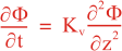
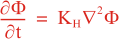
Following Weaver and Courtier (2001), the vertical and horizontal correlations, C, for any state variable Φ are modeled using separated 1D and 2D diffusion equations:

where K_v and K_H are the vertical and horizontal diffusion coefficients (m²/s), assumed to be of order one. They are set to unity (isotropic correlations), if these coefficients are not found in ROMS/TOMS background/model standard deviation NetCDF file (STDname, variables K_v and K_h). The user can set K_v and K_h to the desired patterns to get anisotropic correlations. If we discretize the above diffusion operators using an explicit FTCS scheme, the stability limit is governed by:

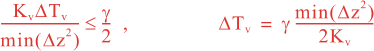
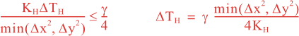
In practice, we set γ < 1 to be below the stability threshold, (γ = 0.5). This stability parameter is set in 4DVAR input script. There are two variables: Vgamma and Hgamma for vertical and horizontal diffusion operators. In realistic applications, the vertical difussion needs to be solved implicitly (IMPLICIT_VCONV). Otherwise, the it will be very expensive since the vertical scales are much smaller. The implicit algorithm is unconditionally stable for any time-step, so we use the maximum thickness in the above equation instead of the minimum.

The parameters controlling the vertical and horizontal length-scales of the Gaussian correlation function are:

over a time interval 0 ≤ t ≤ T and

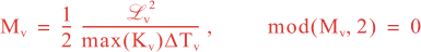
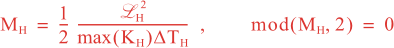
where M_v and M_H are the total number of vertical and horizontal integration steps. Notice that both values are forced to an even number since the squared-root diffusion operators are used to insure symmetry. The squared-root operator iterates only for half of the steps. For any given decorrelation length-scale, the number of integration steps are given by:

The vertical and horizontal decorrelation scales (m) are set in 4DVar input script variables Vdecay(:) and Hdecay(:) for each state variable.

ROMS/TOMS reports to standard output all the parameters associated with these diffusion operators. For example,

 5.0000E-01  Hgamma          Horizontal diffusion stability/accuracy factor.
 5.0000E-05  Vgamma          Vertical diffusion stability/accuracy factor.
  20000.000  Hdecay(isFsur)  Horizontal decorrelation scale (m), free-sruface.
  20000.000  Hdecay(isUbar)  Horizontal decorrelation scale (m), 2D U-momentum.
  20000.000  Hdecay(isVbar)  Horizontal decorrelation scale (m), 2D V-momentum.
  20000.000  Hdecay(isUvel)  Horizontal decorrelation scale (m), 3D U-momentum.
  20000.000  Hdecay(isVvel)  Horizontal decorrelation scale (m), 3D V-momentum.
  20000.000  Hdecay(idTvar)  Horizontal decorrelation scale (m), temp.
  20000.000  Hdecay(idTvar)  Horizontal decorrelation scale (m), salt.
      5.000  Vdecay(isUvel)  Vertical decorrelation scale (m), 3D U-momentum.
      5.000  Vdecay(isVvel)  Vertical decorrelation scale (m), 3D V-momentum.
      5.000  Vdecay(idTvar)  Vertical decorrelation scale (m), temp.
      5.000  Vdecay(idTvar)  Vertical decorrelation scale (m), salt.

 Minimum X-grid spacing, DXmin =  5.26835784E+00 km
 Maximum X-grid spacing, DXmax =  5.58390264E+00 km
 Minimum Y-grid spacing, DYmin =  5.05224079E+00 km
 Maximum Y-grid spacing, DYmax =  5.35460591E+00 km
 Minimum Z-grid spacing, DZmin =  1.33333333E-01 m
 Maximum Z-grid spacing, DZmax =  2.86550363E+02 m

 Minimum barotropic Courant Number =  2.99123135E-02
 Maximum barotropic Courant Number =  8.17259140E-01
 Maximum Coriolis   Courant Number =  3.43845829E-02

 Horizontal convolution, NHsteps, DTsizeH =    64  3.19064213E+06 s  zeta
 Horizontal convolution, NHsteps, DTsizeH =    64  3.19064213E+06 s  ubar
 Horizontal convolution, NHsteps, DTsizeH =    64  3.19064213E+06 s  vbar
 Horizontal convolution, NHsteps, DTsizeH =    64  3.19064213E+06 s  u
 Horizontal convolution, NHsteps, DTsizeH =    64  3.19064213E+06 s  v
 Horizontal convolution, NHsteps, DTsizeH =    64  3.19064213E+06 s  temp
 Horizontal convolution, NHsteps, DTsizeH =    64  3.19064213E+06 s  salt

 Vertical   convolution, NVsteps, DTsizeV =     6  2.05277776E+00 s  u
 Vertical   convolution, NVsteps, DTsizeV =     6  2.05277776E+00 s  v
 Vertical   convolution, NVsteps, DTsizeV =     6  2.05277776E+00 s  temp
 Vertical   convolution, NVsteps, DTsizeV =     6  2.05277776E+00 s  salt

It is recommended to reduce the Vgamma parameter until a value of M_v is around six for vertical diffusion accuracy.

The incremental, strong contraint 4DVAR (IS4DVAR) approximated approach was proposed by Courtier et al. (1994) to reduce the computational cost and facilitate better preconditioning. We follow the algorithm proposed by Weaver et al (2002) that defines the increment to the difference from previous reference state.

Let x^k denote the state vector on the k-th outer loop such that δx^k is the increment difference from the previous state

where x^{k -1} is the current estimate of the ocean state. It is equal to the background state for the first minimization (x⁰ = x_b, δx¹ = 0). The cost function on the k-th loop can be written as

where d^{k – 1} = x_o – Hx^{k – 1} is the innovation vector, x_o is the observation vector, x_b is the background state, H is a linear approximation of the observation operator H, and B and O are the background and observation error covariance matrices. Let’s introduce a new minimization variable δv, such that:

It is more convenient to work in terms of δv (minimization space: v-space). The conditioning of the J_b in v-space is optimal since it’s Hessian, ∂²J_b/∂v², yields the identity matrix. The gradient of J in v-space, denoted ∇_vJ, is given by:

where B = B^T/2B^1/2 and B^T/2 denotes (B^1/2)^T, and ∇_xJ_o is the gradient of J_o in model space (x-space) which is computed using the adjoint model and given by:

Following Weaver and Courtier (2001), the background-error covariance matrix can be factored as:

where S is a diagonal matrix of background-error standard deviations, C is a symetric matrix of background-error correlations which can be factorized as C = C^1/2C^T/2, G is the normalization matrix which ensures that the diagonal elements of C are equal to unity, L is a 3D self-adjoint filtering operator, and W is the grid cell area (2D fields) or volume (3D fields).